Mock Observations (cookbook)

Mera ships a full mock-observation toolkit — beam/PSF convolution, velocity cubes and moment maps, position–velocity diagrams, spectra, emission maps, and FITS export. This page ties them together with the auto-frame: orient the galaxy once, then reuse that frame to produce the image and the kinematics, exactly as a telescope would see them.

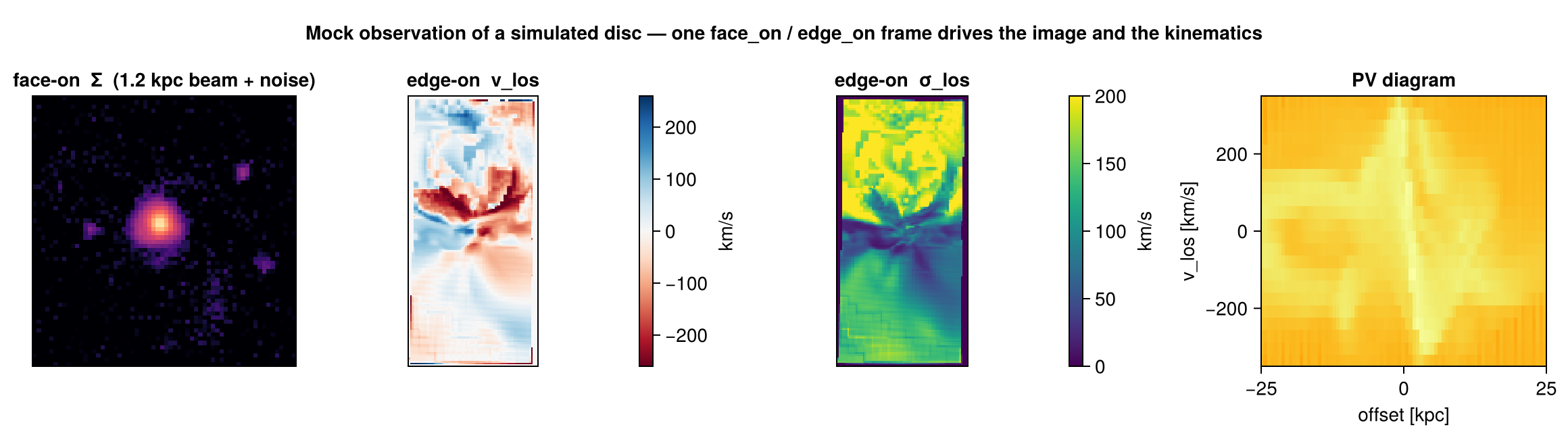
From one simulated disc: a face-on surface-density image with a finite beam and noise, an edge-on line-of-sight velocity field, its dispersion, and a position–velocity diagram — all from a single face_on/edge_on frame.

The rule of thumb the figure follows: face-on for morphology, edge-on for kinematics (a disc's rotation is in its plane, so it shows up along the line of sight only when the disc is tilted toward edge-on).

Step 0 — orient once, reuse everywhere

face_on / edge_on return a frame whose los/up/center feed every function below. Compute it once so the image and the kinematics share the same geometry:

using Mera
gas = gethydro(getinfo(100, "/data/Mera-Tests/spiral_clumps"))

fo = face_on(gas; aperture=0.3)     # disc spin axis (aperture isolates the disc)
eo = edge_on(gas; aperture=0.3)
view = (; center=fo.center, range_unit=fo.center_unit,
          xrange=[-0.22, 0.22], yrange=[-0.22, 0.22])   # zoom onto the disc

(For a crowded or cosmological box, give face_on a seed center + aperture so it locks onto one object — see Auto-Frame.)

Step 1 — a mock image (beam/PSF + noise)

Project the quantity, then convolve with a beam and add noise via mock_observe:

pr  = projection(gas, :sd; los=fo.los, up=fo.up, view...)
img = mock_observe(pr, :sd; beam_fwhm=1.2, beam_unit=:kpc,          # a physical beam …
                   noise=0.004*maximum(pr.maps[:sd]), rng=MersenneTwister(1))

The beam can also be angular — give beam_unit=:arcsec (or :arcmin/:deg) together with a source distance; the physical beam is then θ × distance (small-angle). Use Mera's cosmology helpers for the angular-diameter distance of a redshifted source. A seeded rng makes the noise reproducible.

Step 2 — velocity field and dispersion (moment maps)

velocity_cube builds a spectral (velocity-channel) cube along the line of sight; velocity_moments collapses it to the moment-0/1/2 maps Σ, vlos, σlos:

vc = velocity_cube(gas; los=eo.los, up=eo.up, view...,
                   nv=90, vrange=[-350, 350], v_unit=:km_s)
m  = velocity_moments(vc)        # m.Σ (column), m.vlos (rotation), m.σlos (dispersion)

vrange acts like a spectrometer bandwidth — windowing out high-velocity outliers. The binned σlos is biased slightly high for under-resolved lines (Sheppard correction); for a bias-free velocity or dispersion map of any vector, use los_component(gas, (:vx,:vy,:vz); dispersion=true), which accumulates the moments from the continuous per-cell samples.

Step 3 — position–velocity diagram

position_velocity bins mass into (offset along an in-plane axis, line-of-sight velocity) — the classic long-slit / PV kinematic diagnostic:

pv = position_velocity(gas; los=eo.los, up=eo.up,
                       center=fo.center, range_unit=fo.center_unit,
                       nbins=160, offset_unit=:kpc, v_unit=:km_s)
# pv.offset, pv.velocity (bin edges), pv.pv (the nbins×nbins mass map)

Step 4 — spectra and emission

getspectrum(vc; x=0, y=0) returns the line-of-sight spectrum through a sky pixel (a synthetic emission-line profile from a velocity cube; a PDF from a los_cube(:T)).
integrated_spectrum(vc) sums it over the whole map — the global line profile.
emission_map(gas; kappa, source) makes an optical-depth-weighted emission map (an absorption/emission line image) rather than a plain column.

Step 5 — export to FITS / cubes

savefits writes a map or cube to FITS with a WCS (linear or sky), so it opens in DS9 / astropy / CASA. It is a package extension — using FITSIO first.
savecube / loadcube round-trip a velocity cube via JLD2.