Gravity Data: First Inspection

This notebook provides a comprehensive introduction to loading and analyzing gravitational field data using Mera.jl. You'll learn the fundamentals of working with RAMSES gravity data and its relationship to AMR (Adaptive Mesh Refinement) structures.

Learning Objectives

• Load and inspect gravitational simulation data
• Understand gravitational potential and acceleration field organization
• Analyze gravity data distributions across AMR levels
• Handle different gravity variable types and unit conversions
• Work with IndexedTables data structures for gravity field analysis
• Apply memory management best practices for gravity data

Quick Reference: Essential Gravity Functions

This section provides a comprehensive reference of key Mera.jl functions for gravity data analysis.

Data Loading Functions

# Load simulation metadata with gravity information
info = getinfo(output_number, "path/to/simulation")
info = getinfo(300, "/path/to/sim")                   # Specific output
info = getinfo("/path/to/sim")                        # Latest output

# Load gravity data - basic usage
grav = getgravity(info)                               # Load all variables, all levels

Data Exploration Functions

# Analyze data structure and properties
overview_amr = amroverview(grav)                      # AMR grid structure analysis
data_overview = dataoverview(grav)                   # Statistical overview of variables
usedmemory(grav)                                      # Memory usage analysis

# Explore object structure
viewfields(grav)                                      # View GravDataType structure
viewfields(info.descriptor)                          # View descriptor properties
propertynames(grav)                                   # List all available fields

Variable and Descriptor Management

# Access and modify variable descriptors
info.descriptor.gravity                               # Current gravity variable names
info.descriptor.gravity[2] = :accel_x                # Customize variable names
propertynames(info.descriptor)                       # All descriptor properties

# Access predefined variables (always available)
# :epot (gravitational potential field), :ax, :ay, :az (acceleration components)

IndexedTables Operations

# Work with gravity data tables
using Mera.IndexedTables

# Select specific columns
select(grav.data, (:level, :cx, :cy, :cz, :epot))    # View coordinates + potential
select(data_overview, (:level, :epot_min, :epot_max, :epot_tot)) # Statistical summary

# Extract column data
column(data_overview, :epot_tot)                     # Extract total potential as array
column(data_overview, :epot_min) * info.scale.J_g    # Convert with scaling

# Transform data in-place
transform(data_overview, :epot_tot => :epot_tot => value->value * info.scale.J_g)

Unit Conversion

# Access scaling factors
scale = grav.scale                                    # Shortcut to scaling factors
constants = grav.info.constants                      # Physical constants

# Common unit conversions for gravity data
potential_physical = grav.data.epot * scale.J_g      # Potential field to J/g
accel_cms2 = grav.data.ax * scale.cm_s2              # Acceleration to cm/s²
force_dyn = mass_g * grav.data.ax * scale.cm_s2      # Force in dynes

Memory Management

# Monitor and optimize memory usage
usedmemory(grav)                                      # Check current memory usage
grav = nothing; GC.gc()                              # Clear variable and garbage collect

Common Analysis Workflow

# Standard gravity data analysis workflow
info = getinfo(300, "/path/to/simulation")           # Load simulation metadata
grav = getgravity(info)                              # Load gravity data
usedmemory(grav)                                      # Check memory usage

# Analyze structure and properties
amr_overview = amroverview(grav)                      # AMR grid analysis
data_overview = dataoverview(grav)                   # Variable statistics
viewfields(grav)                                      # Explore data structure

# Convert units and extract specific data
scale = grav.scale                                    # Create scaling shortcut
potential_jg = select(grav.data, :epot) * scale.J_g  # Physical potential field
field_dist = select(data_overview, (:level, :epot_tot)) # Potential distribution by level

Package Import and Initial Setup

Let's start by importing Mera.jl and loading simulation information for output 300:

using Mera
info = getinfo(300, "/Volumes/FASTStorage/Simulations/Mera-Tests/mw_L10");

[Mera]: 2026-06-01T14:04:42.105
Code: RAMSES
output [300] summary:
mtime: 2023-04-09T05:34:09
ctime: 2025-06-21T18:31:24.020
=======================================================
simulation time: 445.89 [Myr]
boxlen: 48.0 [kpc]
ncpu: 640
ndim: 3
cosmological:  false
-------------------------------------------------------
amr:           true
level(s): 6 - 10 --> cellsize(s): 750.0 [pc] - 46.88 [pc]
-------------------------------------------------------
hydro:         true
hydro-variables:
7  --> (:rho, :vx, :vy, :vz, :p, :scalar_00, :scalar_01)
hydro-descriptor: (:density, :velocity_x, :velocity_y, :velocity_z, :pressure, :scalar_00, :scalar_01)
γ: 1.6667
-------------------------------------------------------
gravity:       true
gravity-variables: (:epot, :ax, :ay, :az)
-------------------------------------------------------
particles:     true
- Nstars:   5.445150e+05
particle-variables:
7  --> (:vx, :vy, :vz, :mass, :family, :tag, :birth)
particle-descriptor: (:position_x, :position_y, :position_z, :velocity_x, :velocity_y, :velocity_z, :mass, :identity, :levelp, :family, :tag, :birth_time)
-------------------------------------------------------
rt:            false
clumps:           false
-------------------------------------------------------
namelist-file:
("&COOLING_PARAMS", "&SF_PARAMS", "&AMR_PARAMS", "&BOUNDARY_PARAMS", "&OUTPUT_PARAMS", "&POISSON_PARAMS", "&RUN_PARAMS", "&FEEDBACK_PARAMS", "&HYDRO_PARAMS", "&INIT_PARAMS", "&REFINE_PARAMS")
-------------------------------------------------------
timer-file:       true
compilation-file: false
makefile:         true
patchfile:        true
=======================================================

Understanding Gravity Properties

The output above provides a comprehensive overview of the loaded gravity data properties:

• Gravity files status - Confirms existence and accessibility of gravity data files
• Variable count - Shows the number of predefined and available gravity variables
• Variable names - Lists the gravity variable names from the RAMSES descriptor file
• Data organization - Reveals how the gravity data is structured and stored

Variable Names and Descriptors

Predefined Variable Names: Mera.jl recognizes standard gravity variable names such as :epot, :ax, :ay, :az. These provide a consistent interface for accessing gravitational field quantities across different simulations.

Core Variables:

• :epot - Gravitational potential field (φ)
• :ax, :ay, :az - Gravitational acceleration components

Custom Variable Descriptors: In future versions, you will be able to use variable names directly from the gravity descriptor by setting info.descriptor.usegravity = true. Currently, you can customize variable names by modifying the descriptor array manually.

Let's examine the current gravity descriptor configuration:

info.descriptor.gravity

4-element Vector{Symbol}:
 :epot
 :ax
 :ay
 :az

Customizing Variable Names

You can modify variable names in the descriptor to better match your simulation setup or personal preferences. For example, changing the second gravity variable to a more descriptive name:

info.descriptor.gravity[2] = :a_x;

info.descriptor.gravity

4-element Vector{Symbol}:
 :epot
 :a_x
 :ay
 :az

Exploring Descriptor Properties

Let's examine the complete structure of the descriptor object to understand all available configuration options:

viewfields(info.descriptor)

[Mera]: Descriptor overview
=================================
hversion	= 1
hydro
	= [:density, :velocity_x, :velocity_y, :velocity_z, :pressure, :scalar_00, :scalar_01]
htypes	= ["d", "d", "d", "d", "d", "d", "d"]
usehydro	=
false
hydrofile	= true
pversion	= 1
particles	= [:position_x, :position_y, :position_z, :velocity_x, :velocity_y, :velocity_z, :mass, :identity, :levelp, :family, :tag, :birth_time]
ptypes	= ["d", "d", "d", "d", "d", "d", "d", "i", "i", "b", "b", "d"]
useparticles	= false
particlesfile	= true
gravity	= [:epot, :a_x, :ay, :az]
usegravity	= false
gravityfile	= false
rtversion	= 0
rt
	= Dict{Any, Any}()
rtPhotonGroups	= Dict{Any, Any}()
usert	= false
rtfile	= false
clumps	= Symbol[]
useclumps	= false
clumpsfile	= false
sinks	= Symbol[]
usesinks	= false
sinksfile	= false

For a simple list of all available descriptor fields:

propertynames(info.descriptor)

(:hversion, :hydro, :htypes, :usehydro, :hydrofile, :pversion, :particles, :ptypes, :useparticles, :particlesfile, :gravity, :usegravity, :gravityfile, :rtversion, :rt, :rtPhotonGroups, :usert, :rtfile, :clumps, :useclumps, :clumpsfile, :sinks, :usesinks, :sinksfile)

Loading Gravity Data

Now that we understand our simulation's structure and variable organization, let's load the actual gravitational field data. We'll use Mera's powerful data loading capabilities to read both the gravity field components and their associated AMR grid structure.

Data Loading Overview

The getgravity() function is the primary tool for loading gravitational field data from RAMSES simulations. It provides extensive options for:

• Variable selection - Choose specific gravity quantities (potential, acceleration components)
• Spatial filtering - Focus on regions of interest
• AMR level control - Select refinement levels
• Physical constraints - Set minimum values for AMR cells

Resetting Simulation Information

First, let's reload the simulation information to reset any changes we made to the descriptor:

info = getinfo(300, "/Volumes/FASTStorage/Simulations/Mera-Tests/mw_L10", verbose=false); # here, used to overwrite the previous changes

Loading Complete Gravity Dataset

Now let's load the AMR and gravity data from all files. This will read:

• Full simulation box - All spatial regions
• All gravity variables - Gravitational potential and acceleration components
• All AMR levels - Complete refinement hierarchy
• Cell positions - Only leaf cells (actual data cells, not parent cells)

grav = getgravity(info);

[Mera]: Get gravity data: 2026-06-01T14:04:45.861
Key vars=(:level, :cx, :cy, :cz)
Using var(s)=(1, 2, 3, 4) = (:epot, :ax, :ay, :az)
domain:
xmin::xmax: 0.0 :: 1.0  	==> 0.0 [kpc] :: 48.0 [kpc]
ymin::ymax: 0.0 :: 1.0  	==> 0.0 [kpc] :: 48.0 [kpc]
zmin::zmax: 0.0 :: 1.0  	==> 0.0 [kpc] :: 48.0 [kpc]
📊 Processing Configuration:
   Total CPU files available: 640
   Files to be processed: 640
   Compute threads: 4
   GC threads: 4
Processing files: 100%|██████████████████████████████████████████████████| Time: 0:00:14 (23.26 ms/it)
✓ File processing complete! Combining results...
✓ Data combination complete!
Final data size: 28320979 cells, 4 variables
Creating Table from 28320979 cells with max 4 threads...
   Threading: 4 threads for 8 columns
   Max threads requested: 4
   Available threads: 4
   Using parallel processing with 4 threads
   Creating IndexedTable with 8 columns...
  3.940050 seconds (4.70 M allocations: 4.085 GiB, 0.71% gc time, 23.13% compilation time)
✓ Table created in 4.21 seconds
Memory used for data table :
1.6880627572536469 GB
-------------------------------------------------------

Memory Usage Analysis

The memory consumption of the loaded data is displayed automatically. For detailed memory analysis of any object, Mera.jl provides the usedmemory() function:

usedmemory(grav);

Memory used: 1.688 GB

Understanding Data Types

The loaded data object is now of type GravDataType, which is specifically designed for gravitational field simulation data:

typeof(grav)

GravDataType

Type Hierarchy

GravDataType is part of a well-organized type hierarchy. It's a sub-type of DataSetType:

# Which in turn is a subtype of the general `DataSetType`.
supertype( GravDataType )

DataSetType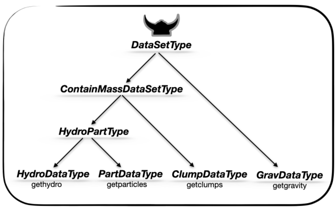

Data Organization and Structure

The gravity data is stored in an IndexedTables table format, with user-selected variables and parameters organized into accessible fields. Let's explore the structure:

viewfields(grav)

data ==> IndexedTables: (:level, :cx, :cy, :cz, :epot, :ax, :ay, :az)
info ==> subfields: (:output, :path, :fnames, :simcode, :mtime, :ctime, :ncpu, :ndim, :levelmin, :levelmax, :boxlen, :time, :aexp, :H0, :omega_m, :omega_l, :omega_k, :omega_b, :unit_l, :unit_d, :unit_m, :unit_v, :unit_t, :gamma, :hydro, :nvarh, :nvarp, :nvarrt, :variable_list, :gravity_variable_list, :particles_variable_list, :rt_variable_list, :clumps_variable_list, :sinks_variable_list, :descriptor, :amr, :gravity, :particles, :rt, :clumps, :sinks, :namelist, :namelist_content, :headerfile, :makefile, :files_content, :timerfile, :compilationfile, :patchfile, :Narraysize, :scale, :grid_info, :part_info, :compilation, :constants)
lmin	= 6
lmax	= 10
boxlen	= 48.0
ranges	=
[0.0, 1.0, 0.0, 1.0, 0.0, 1.0]
selected_gravvars	= [1, 2, 3, 4]
scale ==> subfields: (:Mpc, :kpc, :pc, :mpc, :ly, :Au, :km, :m, :cm, :mm, :μm, :Mpc3, :kpc3, :pc3, :mpc3, :ly3, :Au3, :km3, :m3, :cm3, :mm3, :μm3, :Msol_pc3, :Msun_pc3, :g_cm3, :Msol_pc2, :Msun_pc2, :g_cm2, :Gyr, :Myr, :yr, :s, :ms, :Msol, :Msun, :Mearth, :Mjupiter, :g, :km_s, :m_s, :cm_s, :nH, :erg, :g_cms2, :T_mu, :K_mu, :T, :K, :Ba, :g_cm_s2, :p_kB, :K_cm3, :erg_g_K, :keV_cm2, :erg_K, :J_K, :erg_cm3_K, :J_m3_K, :kB_per_particle, :J_s, :g_cm2_s, :kg_m2_s, :Gauss, :muG, :microG, :Tesla, :eV, :keV, :MeV, :erg_s, :Lsol, :Lsun, :cm_3, :pc_3, :n_e, :erg_g_s, :erg_cm3_s, :erg_cm2_s, :Jy, :mJy, :microJy, :atoms_cm2, :NH_cm2, :cm_s2, :m_s2, :km_s2, :pc_Myr2, :erg_g, :J_kg, :km2_s2, :u_grav, :erg_cell, :dyne, :s_2, :lambda_J, :M_J, :t_ff, :alpha_vir, :delta_rho, :a_mag, :v_esc, :ax, :ay, :az, :epot, :a_magnitude, :escape_speed, :gravitational_redshift, :gravitational_energy_density, :gravitational_binding_energy, :total_binding_energy, :specific_gravitational_energy, :gravitational_work, :jeans_length_grav
ity, :jeans_mass_gravity, :jeansmass, :freefall_time_gravity, :ekin, :etherm, :virial_parameter_local, :Fg, :poisson_source, :ar_cylinder, :aϕ_cylinder, :ar_sphere, :aθ_sphere, :aϕ_sphere, :r_cylinder, :r_sphere, :ϕ, :dimensionless, :rad, :deg)

Convenient Data Access

For convenience, all fields from the original InfoType object are now accessible through:

• grav.info - All simulation metadata and parameters
• grav.scale - Scaling relations for converting from code units to physical units

The data object also retains important structural information:

• Minimum and maximum AMR levels of the loaded data
• Box dimensions and coordinate ranges
• Selected spatial regions and filtering parameters
• Number and properties of loaded gravity variables

Quick Field Reference

For a simple list of all available fields in the gravity data object:

propertynames(grav)

(:data, :info, :lmin, :lmax, :boxlen, :ranges, :selected_gravvars, :used_descriptors, :scale)

Data Analysis and Exploration

Now that we have loaded our gravity data, let's explore its structure and properties in detail. This section demonstrates the key analysis functions available in Mera.jl.

Analysis Overview

We'll cover two main types of analysis:

• AMR Structure Analysis - Understanding the adaptive mesh refinement hierarchy and how gravitational fields are organized across refinement levels, analyzing spatial distribution of field data

• Statistical Data Overview - Computing basic statistical properties of gravity variables, understanding potential and acceleration field distributions, ranges, and assessing data quality

AMR Grid Structure Analysis

The amroverview() function provides detailed information about the adaptive mesh refinement structure associated with our gravity data. The analysis includes:

• Level distribution - Number of cells at each refinement level

The results are returned as an IndexedTables table in code units, ready for further analysis:

overview_amr = amroverview(grav)

Counting...

Table with 5 rows, 3 columns:
level  cells     cellsize
─────────────────────────
6      66568     0.75
7      374908    0.375
8      7806793   0.1875
9      12774134  0.09375
10     7298576   0.046875

Statistical Data Analysis

The dataoverview() function computes comprehensive statistics for all gravity variables in our dataset. This analysis provides:

• Variable ranges - Minimum and maximum values for gravitational potential and acceleration components

The calculated information is stored in code units and can be accessed for further analysis:

data_overview = dataoverview(grav)

Calculating...

Table with 5 rows, 10 columns:
Columns:
#   colname   type
──────────────────
1   level     Any
2   epot_tot  Any
3   epot_min  Any
4   epot_max  Any
5   ax_min    Any
6   ax_max    Any
7   ay_min    Any
8   ay_max    Any
9   az_min    Any
10  az_max    Any

Working with IndexedTables

When dealing with tables containing many columns, only a summary view is typically displayed. To access specific columns, use the select() function.

Important Notes:

• Column names are specified as quoted Symbols (:column_name)
• For more details, see the Julia documentation on Symbols
• The select() function maintains data order and relationships

Let's select specific columns to examine level-wise potential statistics:

using Mera.IndexedTables # to import the IndexedTables package, which is a dependency of Mera

select(data_overview, (:level,:epot_tot, :epot_min, :epot_max ) )

Table with 5 rows, 4 columns:
level  epot_tot    epot_min   epot_max
───────────────────────────────────────
6      -9309.98    -0.157858  -0.105458
7      -61891.4    -0.175757  -0.151563
8      -1.66608e6  -0.292519  -0.172968
9      -4.35579e6  -0.579801  -0.225363
10     -3.57477e6  -0.986489  -0.271161

Single column Extraction Example

Extract total potential data from a specific column. The column() function retrieves data from a specific table column, maintaining the order consistent with the table structure:

column(data_overview, :epot_tot)

5-element Vector{Any}:
  -9309.980771585666
 -61891.37272811445
     -1.6660843210800427e6
     -4.355786574891018e6
     -3.5747698183847037e6

Data Structure Deep Dive

Now let's examine the detailed structure of our gravity data. Understanding this organization is crucial for effective data manipulation and analysis.

IndexedTables Storage Format

The gravity data is stored in grav.data as an IndexedTables table (in code units), which provides several key advantages:

• Row-based organization: Each row represents a single cell in the simulation
• Column-based access: Each column represents a specific gravitational field property
• Efficient operations: Built-in support for filtering, mapping, and aggregation
• Memory efficiency: Optimized storage and access patterns for gravitational field data
• Functional interface: Clean, composable operations for data manipulation

For comprehensive information on working with this data structure:

• Mera.jl documentation and tutorials
• JuliaDB API Reference
• IndexedTables.jl documentation

Understanding the Data Layout

The table structure reflects the AMR grid organization:

Spatial Coordinates

• Integer cell positions (cx, cy, cz) form a uniform 3D array within each refinement level
• Level-specific ranges: Each refinement level has its own coordinate system
  • Level 8: coordinates range from 1-256
  • Level 14: coordinates range from 1-16384
• Sparse occupancy: Not all coordinate positions exist due to adaptive refinement

Critical Data Integrity Notes

• Coordinate preservation: The integers cx, cy, cz are essential for grid reconstruction
• Do not modify: These coordinates maintain the AMR spatial relationships
• Unique identifiers: Each (level, cx, cy, cz) combination uniquely identifies a cell

Let's examine the complete data table:

grav.data

Table with 28320979 rows, 8 columns:
level  cx   cy   cz   epot       ax         ay         az
───────────────────────────────────────────────────────────────────
6      1    1    1    -0.105458  0.0713717  0.0713739  0.0714421
6      1    1    2    -0.106574  0.0736603  0.0736626  0.071396
6      1    1    3    -0.107689  0.0759945  0.0759969  0.0712471
6      1    1    4    -0.1088    0.0783709  0.0783733  0.0709879
6      1    1    5    -0.109906  0.0807857  0.0807883  0.0706111
6      1    1    6    -0.111006  0.0832346  0.0832372  0.0701094
6      1    1    7    -0.112097  0.0857126  0.0857152  0.0694754
6      1    1    8    -0.113176  0.0882139  0.0882167  0.068702
6      1    1    9    -0.114243  0.0907326  0.0907354  0.0677824
6      1    1    10   -0.115294  0.0932614  0.0932643  0.0667098
6      1    1    11   -0.116327  0.095793   0.095796   0.0654782
6      1    1    12   -0.117339  0.0983188  0.0983218  0.064082
⋮
10     814  493  514  -0.28418   -0.734355  0.0468811  -0.00847598
10     814  494  509  -0.284171  -0.733368  0.0443188  0.0287892
10     814  494  510  -0.284196  -0.73424   0.0441712  0.0222774
10     814  494  511  -0.284214  -0.734832  0.0441283  0.0151562
10     814  494  512  -0.284225  -0.735242  0.0440921  0.00732157
10     814  494  513  -0.284228  -0.73512   0.0441534  -0.000562456
10     814  494  514  -0.284224  -0.734709  0.0442907  -0.00837105
10     814  495  511  -0.284256  -0.735055  0.0415764  0.0151266
10     814  495  512  -0.284267  -0.73541   0.0415465  0.00732422
10     814  496  511  -0.284295  -0.735248  0.0390693  0.0150688
10     814  496  512  -0.284306  -0.735572  0.0390361  0.00736339

Focused Data Examination

For a more detailed view of specific columns, we can select key fields to understand the gravity data organization better:

select(grav.data, (:level,:cx, :cy, :cz, :epot) )

Table with 28320979 rows, 5 columns:
level  cx   cy   cz   epot
───────────────────────────────
6      1    1    1    -0.105458
6      1    1    2    -0.106574
6      1    1    3    -0.107689
6      1    1    4    -0.1088
6      1    1    5    -0.109906
6      1    1    6    -0.111006
6      1    1    7    -0.112097
6      1    1    8    -0.113176
6      1    1    9    -0.114243
6      1    1    10   -0.115294
6      1    1    11   -0.116327
6      1    1    12   -0.117339
⋮
10     814  493  514  -0.28418
10     814  494  509  -0.284171
10     814  494  510  -0.284196
10     814  494  511  -0.284214
10     814  494  512  -0.284225
10     814  494  513  -0.284228
10     814  494  514  -0.284224
10     814  495  511  -0.284256
10     814  495  512  -0.284267
10     814  496  511  -0.284295
10     814  496  512  -0.284306

Summary and Next Steps

What You've Learned

In this tutorial, you've mastered the fundamentals of working with gravitational field data in Mera.jl:

1. Data Loading: How to load gravity data using getgravity() with various options
2. Structure Understanding: The organization of gravitational field data and its relationship to AMR grids
3. Variable Management: Working with predefined gravity variable names and field components
4. Data Analysis: Using amroverview() and dataoverview() for comprehensive gravity analysis
5. Unit Handling: Converting between code units and physical units for gravitational quantities
6. Memory Management: Monitoring and optimizing memory usage for gravity field datasets
7. Data Manipulation: Using IndexedTables operations for efficient gravity data processing

Key Takeaways

• Gravity data is stored in IndexedTables format for efficient access and manipulation
• AMR coordinates (level, cx, cy, cz) are critical for spatial relationships and should not be modified
• Always be conscious of units - raw data is in code units
• Memory management is crucial for large gravity field datasets
• Gravitational potential and acceleration components provide complementary field information
• Mera.jl provides powerful tools for statistical analysis and gravity data exploration

Continue Your Learning

Now that you understand gravity data fundamentals, you can explore:

• Advanced gravity analysis: Field calculations, force computations, and potential energy analysis
• Multi-component field analysis: Combining potential and acceleration data for comprehensive field studies
• Multi-physics analysis: Combining gravity data with hydro and particle data
• Time series analysis: Working with multiple simulation outputs to study gravitational evolution
• Performance optimization: Advanced techniques for large-scale gravity data processing