MERA.jl
Analyze RAMSES simulations at scale, in pure Julia.

MERA reads and analyzes astrophysical simulation output natively in Julia. It is built for RAMSES: multi-resolution AMR grids carrying hydro and MHD, plus particles, gravity, clumps, sinks and radiative-transfer fields, loaded into memory-efficient tables. Cosmological runs are handled throughout, with scale factor, redshift and the derived quantities that depend on them. It derives quantities on demand, thermodynamics and kinematics, magnetic and gravitational fields, ionisation states, Jeans and virial diagnostics, each in any unit. On top of that it provides conservation-correct projections, on axis or from any viewing angle, radial and vertical profiles, phase diagrams, structure finding, star-formation rates, time series across outputs, animations and VTK export for ParaView, all through one unified, multiple-dispatch API.
Formats are read through a registry rather than hard-wired, so the analysis works on the data and never learns which code produced it. quicklook is the quickest way in: point it at a snapshot you have never seen and it reports what is there and draws it.
Support for AREPO, GADGET, PLUTO, Athena++, FLASH, Chombo and AMReX/Quokka is in active development for version 2.0, on the multicode branch. AMReX/BoxLib is also the container used by Castro, Nyx and WarpX. It is not part of any 1.x release, and nothing on these pages depends on it.
For collaborators who want to try it:
] add https://github.com/ManuelBehrendt/Mera.jl#multicodeThose readers are newer and narrower than the RAMSES one and are tested mainly against synthetic fixtures. Widening that is mostly reader work rather than core work, because the analysis layer is code-blind, so contributions and bug reports move it forward quickly.
Computational astrophysicist analyzing AMR simulation data with MERA.jl's powerful visualization and analysis capabilities
Start here
Install the package:
using Pkg
Pkg.add("Mera")
using Mera
Then run something on a real RAMSES simulation. download_testdata fetches one of Mera's public test simulations and hands you the path:
using Mera, CairoMakie
path = download_testdata("stromgren3d")   # a source ionising neutral gas
info = getinfo(path, output=7)            # the last of its seven snapshots
gas  = gethydro(info)
p    = projection(gas, :xHII)             # the ionised-hydrogen fraction

heatmap(p.extent[1:2], p.extent[3:4], p.maps[:xHII]; colormap=:inferno)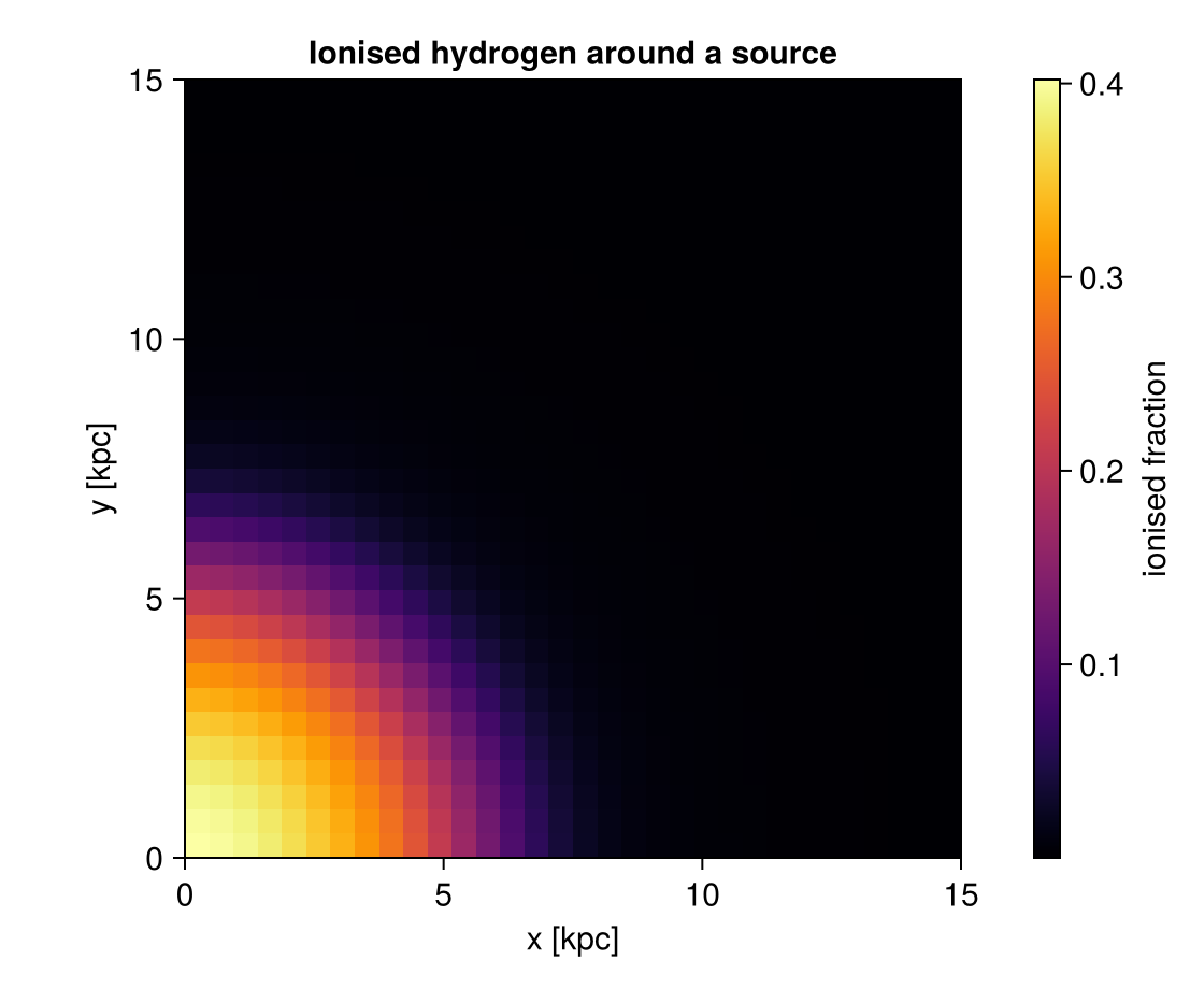
projection returns an object rather than a picture: the map is p.maps[:xHII] and its edges are p.extent, in kpc here, so you can draw it with any plotting package. Mera draws nothing itself.
The source sits at a corner of the box and ionises outward, so the run follows one octant of the sphere at eight times the effective resolution. Its answer is known: the ionisation front should follow the Strömgren law, which is what Mera's own test suite checks it against.
With a simulation of your own, point getinfo at the output folder and continue the same way:
info = getinfo(300, "/path/to/simulation")   # reads output_00300
gas  = gethydro(info)
Loading several components means writing the same selection on each call. One call does all of it, and the same line works on a converted MERA file:
(; hydro, particles, info) = loadall("/path/to/simulation", 300;
                                     lmax=10, xrange=[-10., 10.],
                                     center=[:bc], range_unit=:kpc)
See Pipelines for that, for the matching projection shorthand, and for keeping one selection in step across a whole script.
Once you are past the tutorials, the Gallery holds complete workflows you can point at your own simulation, and is where to share the analysis behind a paper.
If you are working with an AI assistant, Using an AI Assistant has a short file to give it so that it writes Mera that runs, and the three checks worth keeping in any script it produces. It is an experiment rather than a policy.
Where to start is the other way in: one table from "I want to …" to the function that does it, for the twenty things people reach for first.
Next: First Look. It shows what one command tells you about an unfamiliar output, and what it costs on a large one. From there the sidebar follows the order you will actually work in: inspect, load, select, compute, project.
Installing the plotting packages
Mera itself draws nothing. The tutorials plot with CairoMakie, and a few of the older projection pages use PyPlot. Neither is a Mera dependency, so add whichever you need before running a page that plots:
Pkg.add("CairoMakie")   # what most tutorial figures use
Pkg.add("PyPlot")       # only the projection pages that import it
Mera's Makie support ships as a package extension: it activates by itself once a Makie backend such as CairoMakie is loaded, with nothing further to install.
For the wider ecosystem around a Mera workflow, tables, units, statistics and IO, see Recommended Packages.
Requirements: Julia 1.10 or newer, 1.12+ recommended, and 8GB+ RAM Platforms: macOS (including Apple Silicon), Linux, Windows Tested on every push: Julia 1.10 / 1.11 / 1.12 / 1.13 × Linux, macOS and Windows, twelve jobs
Julia 1.10 is the minimum the package supports (julia = "1.10" in Project.toml) and stays in CI so it keeps working. 1.12 is what we recommend running: the compiler is faster and the garbage collector handles the large allocations of AMR and particle analysis better, which is most of what Mera does. CI runners have no simulation data, so they exercise the data-free tiers: the synthetic-HDF5 reader contracts, the reader registry, the IO layer and the mera-file round-trips, while the full suite runs against real snapshots locally, on one configuration: Julia 1.12 on macOS (Apple Silicon). The data-backed tier is therefore verified on a single platform, not across the whole matrix.
What Mera gives you
One API across data types. Mera reads six: hydro, particles, gravity, clumps, sinks and radiative transfer. MHD is not a seventh, the magnetic field arrives as extra columns on hydro. The same function name works on each, and Julia's multiple dispatch selects the right method, so you write the analysis once:
getvar(gas,       :mass)     # cell mass, density times volume
getvar(particles, :mass)     # particle mass, discrete values
getvar(clumps,    :mass)     # clump mass, one row per clump
getvar(sinks,     :mass)     # sink mass, the column RAMSES calls msink

getvar(gravity,   :epot)     # gravity carries a potential, not a mass
getvar(rt,        :Np1)      # photon density of group 1
getvar(gas,       :bx)       # MHD, as a field on the hydro cells

projection(gas,       :rho)  # gas density
projection(particles, :age)  # stellar age distribution
projection(rt,        :Np1)  # photon density, through the same engine
Dispatch picks the method, it does not invent physics: a quantity exists where it means something. :mass is defined for gas, particles, clumps and sinks, while gravity and RT carry fields instead. Projection covers the types laid out on the AMR grid and the particles, so clumps and sinks, which are catalogues of points, are analysed through regions and getvar rather than projected.
AMR handled correctly. Multi-resolution grids are read natively from the RAMSES binary format, with Hilbert space-filling curve support, correct level weighting, and projections that conserve mass across refinement boundaries.
One table, one row per cell. Mera holds a snapshot as a table: one contiguous column per quantity, sorted on the cell's grid address (level, cx, cy, cz). Three things follow, and they are why the rest of this page is possible.
The refinement level travels with every cell, so nothing has to be resampled onto a uniform grid first. A projection deposits each cell at its own size in a single pass over all levels, and :level can be selected on like any physical quantity.
Selecting is cheap. A mask picks rows as views rather than copying columns, so a cut costs the columns you actually read and not the whole table. You can select in value space on anything getvar computes, in any unit, and combine those conditions: filterdata(gas, Above(:T, 1e4, :K) & Below(:rho, 1e3, :nH)).
Results stay the same kind of thing. A region or a filter hands back an object of the original type, so subregion into filterdata into projection into getvar chains without adapters or conversions.
Built for large outputs on ordinary machines. Selective loading keeps memory in hand, and the numbers are measured rather than assumed. Convert a snapshot once with savedata and reading it back is the same data, far cheaper:
| reading one snapshot, all components | from the RAMSES output | from the MERA file |
|---|---|---|
| time | 514.9 s | 22.7 s |
| memory allocated | 665.4 GB | 47.4 GB |
| size on disk | 53.18 GB | 12.73 GB |
A production run with 5120 CPU files and 20489 files on disk, read at full resolution. The gain comes from not re-parsing every Fortran file and not storing the AMR hierarchy, so it grows with the file count and depends on your simulation. Performance has the method, the limits, and the raw reports.
Physics on demand. Nothing is precomputed and nothing is stored twice: ask for a quantity by name and Mera derives it from what the snapshot actually holds, in the unit you ask for.
| thermodynamics | temperature, sound speed, mean molecular weight, five entropy measures, cooling time and length |
| kinematics | velocities and Mach numbers in Cartesian, cylindrical and spherical frames, and the squared components the dispersions build on |
| magnetic fields | components in three coordinate systems, magnitude, magnetic pressure, plasma beta, Alfvén speed, and Alfvén, fast and slow magnetosonic Mach numbers |
| gravity | potential, accelerations and forces in three coordinate systems, specific and total binding energy |
| stability and star formation | Jeans length, mass and number, local virial parameter, free-fall time |
| angular momentum | specific and total, Cartesian, cylindrical and spherical components |
| radiative transfer | ionisation fractions, number densities, photoionisation and photoheating rates, recombination |
| geometry | cell size and volume, cylindrical and spherical radii, and their minimum-image forms for a periodic box |
| cosmology | overdensity, formation redshift and time, physical age from conformal birth time |
A quantity exists where the data supports it: the magnetosonic Mach numbers need a magnetic field, the ionisation states need radiative transfer. getvar() prints the current list, and add_field adds your own on the same footing.
Cells are split, not counted. Say you want the mass inside a sphere of 10 kpc. The sphere is round. The cells are boxes. Some cells lie half in and half out, and you have to decide what to do with them.
The usual rule looks at the centre of each cell and takes the whole cell or nothing. Mera can keep the part that is really inside:
sph = subregion(gas, sphere(10.))   # 10 kpc around the box centre
msum(sph, :Msol)                    # the mass inside 10 kpc
Every cell on the edge gets a :fraction, a number between 0 and 1, saying how much of it lies inside. getvar(:mass) and getvar(:volume) both use it. This gives you one thing you can rely on: the parts add up to the whole. A sphere of 10 kpc is exactly the 5 kpc sphere plus the shell from 5 to 10 kpc.
How much this changes a number depends on what the edge passes through. Around a large region in ordinary gas the two mistakes, gas wrongly added and gas wrongly dropped, cancel to well under a percent. They stop cancelling when the edge cuts something heavy: in the mw_L10 test galaxy a thin shell with its edge on the densest cell comes out 14 % too heavy. Splitting removes the question, so you do not need to know which case you are in.
That is the arithmetic. The picture is a separate question: a projection spreads each edge cell's fraction-weighted mass over its whole footprint, so a boundary drawn on a coarse patch looks soft. subregion(..., refine_to=[0.05, :kpc]) subdivides the straddling cells until their children are no larger than that, and the rendered edge sharpens to the scale you set. It changes no total, because :fraction already made the totals exact; it is a rendering tool, not an accuracy one.
Only the region values do this, sphere(10.) and the other shapes, and projection with split=true on its depth or fov cut. The xrange/yrange/zrange options when loading, the older style with symbols, and covering_grid all count whole cells. Stars, dark matter and clumps are points, so there is nothing to split. See Subregions.
Results you can defend. Pin versions with a Project.toml and Manifest.toml in your own analysis project, and record what produced each number with provenance. See Reproducibility for how the pieces fit together. VTK export preserves AMR structure for ParaView and VisIt.
Mera supports RAMSES stable-17.09 through stable-19.10, and the 2025.05 and 2026.05 releases. The public test simulations are produced with RAMSES 2026.05 and checked against its own reference solutions on every release, so that support is exercised rather than assumed. Mera is in active use and active development.
About the data in these tutorials
The tutorial pages analyse research-scale RAMSES simulations, several gigabytes each. They are worked examples: read them to see what an analysis of real data looks like, and adapt the code to your own outputs. Those particular simulations are not distributed, so point the examples at a snapshot of your own, or at one of the test simulations below.
To run code as you read, Mera publishes a small set of test simulations, fifteen of them, most a few megabytes (about 300 MB together). Every one carries either an analytic oracle, a law that follows from its own setup, or is checked against reference values published by the RAMSES developers. Mera's own test suite verifies the package against them, so you can confirm an installation behaves correctly. Fetch them all with download_testdata(), or one at a time by name (download_testdata("sedov3d_amr") is 2.3 MB).
Two tutorial pages already use data you can obtain: the radiative-transfer page runs on one of the published test simulations, and the cosmology page carries download instructions for the yt project's public sample dataset.
Three pages need no download at all. Clump Finding: Synthetic Example, Statistics (PDFs) and Uniform Grid / Resampling build their data in memory as they run, and the clump-finding page scores the finder against known positions rather than eyeballing the result.
Every tutorial builds its paths from one variable, so you do not have to edit the cells. Point it at your own simulations and the examples run against them:
ENV["MERA_EXAMPLES"] = "/path/to/your/simulations" # before `using Mera`Where to go next
If you already know what you want to compute:
| you want to | go to |
|---|---|
| see what is in an unfamiliar output | First Look |
| learn the objects and the units | First Steps |
| make a density map | Projections |
| load only part of a large output | Load by Selection |
| cut out a spatial region | Get Subregions |
| compute masses and other quantities | Basic Calculations |
| store or share a snapshot | MERA Files |
| make it faster | Multi-Threading |
| know what it costs before you run it | Performance |
| look up a function | Complete API |
Coming from another analysis tool, or new to Julia:
- Coming from Other Tools, a concept-to-verb mapping, one complete worked workflow, and the differences to expect, stated honestly
- Julia for Simulation Analysis, environments, compile latency, memory and threads, scoped to this kind of work
- Troubleshooting, the first-hour errors, listed under the message Mera actually prints
Citation
If you use MERA in your research, please cite it using the DOI badge above. This supports continued development and helps other researchers discover the tool. Click the badge for BibTeX format. Please also star the GitHub repository.
Community and support
- GitHub Discussions: ask questions, share tips, get help
- Show and Tell: share your scientific results and visualizations
- Report Issues: bug reports and feature requests
- In the REPL:
?getinfofor function docs,methods(getinfo)for available methods - Jupyter notebooks
Ambient Study Music
Ambient Study Music: by MERA, inspired by astrophysics. Eighteen tracks, each named after an astronomical object. Written alongside the package, and meant for long sessions with data.

Spotify · Apple Music · YouTube
License
MIT License, Copyright (c) 2019 Manuel Behrendt.
Permission is hereby granted, free of charge, to any person obtaining a copy of this software and associated documentation files (the "Software"), to deal in the Software without restriction, including without limitation the rights to use, copy, modify, merge, publish, distribute, sublicense, and/or sell copies of the Software, and to permit persons to whom the Software is furnished to do so, subject to the following conditions:
The above copyright notice and this permission notice shall be included in all copies or substantial portions of the Software.
THE SOFTWARE IS PROVIDED "AS IS", WITHOUT WARRANTY OF ANY KIND, EXPRESS OR IMPLIED, INCLUDING BUT NOT LIMITED TO THE WARRANTIES OF MERCHANTABILITY, FITNESS FOR A PARTICULAR PURPOSE AND NONINFRINGEMENT. IN NO EVENT SHALL THE AUTHORS OR COPYRIGHT HOLDERS BE LIABLE FOR ANY CLAIM, DAMAGES OR OTHER LIABILITY, WHETHER IN AN ACTION OF CONTRACT, TORT OR OTHERWISE, ARISING FROM, OUT OF OR IN CONNECTION WITH THE SOFTWARE OR THE USE OR OTHER DEALINGS IN THE SOFTWARE.