3. Clumps: Get Sub-Regions of The Loaded Data

Learning Objectives

By the end of this tutorial, you will be able to:

Extract spatial sub-regions from clump simulation data using geometric selections
Apply cuboid, cylindrical, and spherical filtering to isolate specific regions of interest
Utilize shell regions for hollow geometric selections with inner and outer boundaries
Combine multiple selection criteria for complex spatial filtering operations
Perform inverse selections to analyze data outside specified regions
Visualize selected regions with comprehensive scatter plots and extent analysis

Technical Foundation

Clump Data Structure

Clumps in MERA represent identified overdense regions in simulations, containing:

Spatial coordinates (x, y, z positions)
Physical properties (mass, size, density characteristics)
Hierarchical relationships (parent-child clump associations)
Temporal evolution (formation and merger histories)

Spatial Selection Functions

Core Functions:

subregion() - Primary function for geometric sub-region extraction
shellregion() - Specialized function for hollow region selections
getpositions() - Extract position coordinates with unit conversion
getextent() - Calculate spatial bounds and ranges

Geometric Types:

:cuboid - Rectangular box selections with xrange, yrange, zrange
:cylinder - Cylindrical selections with radius, height, and orientation
:sphere - Spherical selections with radius from center point
:shell - Hollow versions of geometric shapes with inner/outer boundaries

Coordinate Systems:

Standard notation [0:1] - Normalized box coordinates (default)
Physical units - Real length units (kpc, Mpc, pc, etc.)
Center references - :boxcenter, or custom coordinates
Relative positioning - Offsets from specified reference points

Quick Reference

# Basic subregion extraction
subregion(clumps, :cuboid, xrange=[x1,x2], yrange=[y1,y2], zrange=[z1,z2])

# Physical units with custom center
subregion(clumps, :sphere, radius=10.0, center=[5.0, 5.0, 5.0],
          range_unit=:kpc, center_unit=:kpc)

# Cylindrical selection
subregion(clumps, :cylinder, radius=5.0, height=20.0,
          direction=:z, center=[:boxcenter])

# Shell regions (hollow selections)
shellregion(clumps, :sphere, radius=[5.0, 15.0], center=[:boxcenter])

# Position extraction and analysis
x, y, z = getpositions(clumps, :kpc, center=[:boxcenter])
rx, ry, rz = getextent(clumps, :kpc, center=[:boxcenter])

# Inverse selection (data outside region)
subregion(clumps, :cuboid, xrange=[x1,x2], inverse=true)

Data Setup and Initialization

using Mera, PyPlot
rc("figure", dpi=300); rc("savefig", dpi=300)
info = getinfo(400, "/Volumes/FASTStorage/Simulations/Mera-Tests/manu_sim_sf_L14")
clumps = getclumps(info);

[Mera]: 2026-06-01T20:13:56.577
Code: RAMSES
output [400] summary:
mtime: 2018-09-05T09:51:55
ctime: 2025-06-29T20:06:45.267
=======================================================
simulation time: 594.98 [Myr]
boxlen: 48.0 [kpc]
ncpu: 2048
ndim: 3
cosmological:  false
-------------------------------------------------------
amr:           true
level(s): 6 - 14 --> cellsize(s): 750.0 [pc] - 2.93 [pc]
-------------------------------------------------------
hydro:         true
hydro-variables:
7  --> (:rho, :vx, :vy, :vz, :p, :passive_scalar_1, :passive_scalar_2)
hydro-descriptor: (:density, :velocity_x, :velocity_y, :velocity_z, :thermal_pressure, :passive_scalar_1, :passive_scalar_2)
γ: 1.6667
-------------------------------------------------------
gravity:       true
gravity-variables: (:epot, :ax, :ay, :az)
-------------------------------------------------------
particles:     true
- Npart:    5.091500e+05
- Nstars:   5.066030e+05
- Ndm:      2.547000e+03
particle-variables: 5  --> (:vx, :vy, :vz, :mass, :birth)
-------------------------------------------------------
rt:            false
-------------------------------------------------------
clumps:           true
clump-variables: (:index, :lev, :parent, :ncell, :peak_x, :peak_y, :peak_z, Symbol("rho-"), Symbol("rho+"), :rho_av, :mass_cl, :relevance)
-------------------------------------------------------
namelist-file:    false
timer-file:       false
compilation-file: true
makefile:         true
patchfile:        true
=======================================================
[Mera]: Get clump data: 2026-06-01T20:14:00.516
domain:
xmin::xmax: 0.0 :: 1.0  	==> 0.0 [kpc] :: 48.0 [kpc]
ymin::ymax: 0.0 :: 1.0  	==> 0.0 [kpc] :: 48.0 [kpc]
zmin::zmax: 0.0 :: 1.0  	==> 0.0 [kpc] :: 48.0 [kpc]
Read 12 colums:
[:index, :lev, :parent, :ncell, :peak_x, :peak_y, :peak_z, Symbol("rho-"), Symbol("rho+"), :rho_av, :mass_cl, :relevance]
Memory used for data table :
61.58203125 KB
-------------------------------------------------------

Cuboid (rectangular box) selections are the most fundamental geometric filtering method, allowing precise control over data extraction in Cartesian coordinates. This approach is ideal for analyzing specific spatial volumes or comparing different regions within the simulation domain.

Key Features:

Independent axis control - Separate range specification for x, y, z dimensions
Flexible coordinate systems - Standard [0:1] or physical units (kpc, Mpc, etc.)
Custom center references - :boxcenter, or user-defined coordinates
Inverse selection capability - Extract data outside the specified region

Full Domain Visualization

Create scatter plots of the complete simulation box to understand the spatial distribution before applying regional selections.

Use the getvar function to extract the positions of the clumps relative to the box center. It returns a dictionary of arrays:

positions = getvar(clumps, [:x, :y, :z], :kpc, center=[:boxcenter], center_unit=:kpc) # units=[:kpc, :kpc, :kpc]
x, y, z = positions[:x], positions[:y], positions[:z]; # assign the three components of the dictionary to three arrays

Alternatively, use the getposition function to extract the positions of the clumps. It returns a tuple of the three components:

x, y, z = getpositions(clumps, :kpc, center=[:boxcenter], center_unit=:kpc); # assign the three components of the tuple to three arrays

Get the extent of the processed domain with respect to a given center. The returned tuple is useful declare the specific range of the plots.

rx, ry, rz = getextent(clumps, :kpc,  center=[:boxcenter]);

Cuboid Region: The red lines show the region that we want to cut-out as a sub-region from the full data:

figure(figsize=(15.5, 3.5))

subplot(1,3,1)
scatter(x,y)
plot([-4.,0.,0.,-4.,-4.],[-15.,-15.,15.,15.,-15.], color="red")
xlim(rx)
ylim(ry)
xlabel("x k[pc]")
ylabel("y [kpc]")

subplot(1,3,2)
scatter(x,z)
plot([-4.,0.,0.,-4.,-4.],[-2.,-2.,2.,2.,-2.], color="red")
xlim(rx)
ylim(rz)
xlabel("x [kpc]")
ylabel("z [kpc]")

subplot(1,3,3)
scatter(y,z)
plot([-15.,15.,15.,-15.,-15.],[-2.,-2.,2.,2.,-2.], color="red")
xlim(ry)
ylim(rz)
xlabel("y [kpc]")
ylabel("z [kpc]");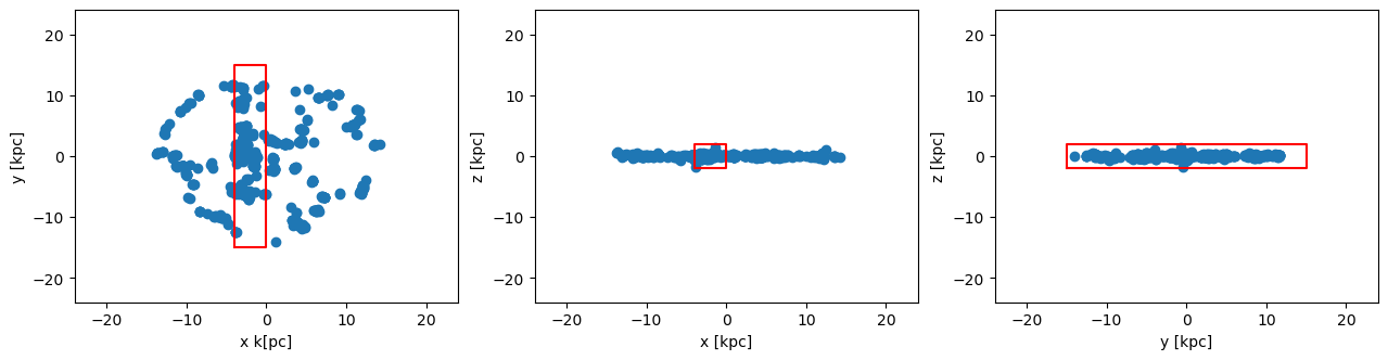

Cuboid Region: Cutout the data assigned to the object `clumps`

Note: The selected regions can be given relative to a user given center or to the box corner [0., 0., 0.] by default. The user can choose between standard notation 0:1 or physical length-units, defined in e.g. info.scale :

clumps_subregion = subregion( clumps, :cuboid,
                                    xrange=[-4., 0.],
                                    yrange=[-15. ,15.],
                                    zrange=[-2. ,2.],
                                    center=[:boxcenter],
                                    range_unit=:kpc);

[Mera]: 2026-06-01T20:14:05.661
center: [0.5, 0.5, 0.5] ==> [24.0 [kpc] :: 24.0 [kpc] :: 24.0 [kpc]]
domain:
xmin::xmax: 0.4166667 :: 0.5  	==> 20.0 [kpc] :: 24.0 [kpc]
ymin::ymax: 0.1875 :: 0.8125  	==> 9.0 [kpc] :: 39.0 [kpc]
zmin::zmax: 0.4583333 :: 0.5416667  	==> 22.0 [kpc] :: 26.0 [kpc]
Memory used for data table :29.33203125
 KB
-------------------------------------------------------

The function subregion creates a new object with the same type as the object created by the function getclumps :

typeof(clumps_subregion)

ClumpDataType

Cuboid Region: Scatter-Plots of the sub-region.

The coordinates center is the center of the box by default:

x, y, z    = getpositions(clumps_subregion, :kpc, center=[:boxcenter]); # clump positions of the subregion
rx, ry, rz = getextent(clumps, :kpc, center=[:boxcenter] ); # extent of the box

figure(figsize=(15.5, 3.5))

subplot(1,3,1)
scatter(x,y)
plot([-4.,0.,0.,-4.,-4.],[-15.,-15.,15.,15.,-15.], color="red")
xlim(rx)
ylim(ry)
xlabel("x k[pc]")
ylabel("y [kpc]")

subplot(1,3,2)
scatter(x,z)
plot([-4.,0.,0.,-4.,-4.],[-2.,-2.,2.,2.,-2.], color="red")
xlim(rx)
ylim(rz)
xlabel("x [kpc]")
ylabel("z [kpc]")

subplot(1,3,3)
scatter(y,z)
plot([-15.,15.,15.,-15.,-15.],[-2.,-2.,2.,2.,-2.], color="red")
xlim(ry)
ylim(rz)
xlabel("y [kpc]")
ylabel("z [kpc]");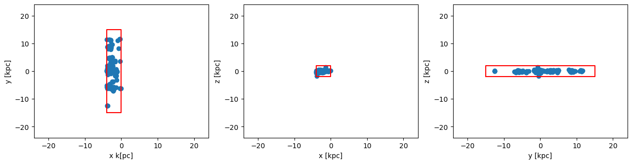

Cuboid Region: Get the extent of the subregion data ranges

rx_sub, ry_sub, rz_sub = getextent(clumps_subregion, :kpc, center=[:boxcenter]); # extent of the subregion

figure(figsize=(15.5, 3.5))

subplot(1,3,1)
scatter(x,y)
xlim(rx_sub)
ylim(ry_sub)
xlabel("x [kpc]")
ylabel("y [kpc]")

subplot(1,3,2)
scatter(x,z)
xlim(rx_sub)
ylim(rz_sub)
xlabel("x [kpc]")
ylabel("z [kpc]")

subplot(1,3,3)
scatter(y,z)
xlim(ry_sub)
ylim(rz_sub)
xlabel("y [kpc]")
ylabel("z [kpc]");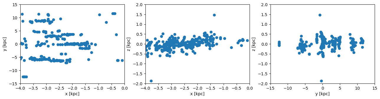

Cuboid Region: Get the data outside of the selected region (inverse selection):

clumps_subregion = subregion( clumps, :cuboid,
                                    xrange=[-4., 0.],
                                    yrange=[-15. ,15.],
                                    zrange=[-2. ,2.],
                                    center=[:boxcenter],
                                    range_unit=:kpc,
                                    inverse=true);

[Mera]: 2026-06-01T20:14:06.556
center: [0.5, 0.5, 0.5] ==> [24.0 [kpc] :: 24.0 [kpc] :: 24.0 [kpc]]
domain:
xmin::xmax: 0.4166667 :: 0.5  	==> 20.0 [kpc] :: 24.0 [kpc]
ymin::ymax: 0.1875 :: 0.8125  	==> 9.0 [kpc] :: 39.0 [kpc]
zmin::zmax: 0.4583333 :: 0.5416667  	==> 22.0 [kpc] :: 26.0 [kpc]
Memory used for data table :33.45703125 KB
-------------------------------------------------------

x, y, z    = getpositions(clumps_subregion, :kpc, center=[:boxcenter]);
rx_sub, ry_sub, rz_sub = getextent(clumps_subregion, :kpc, center=[:boxcenter]);

figure(figsize=(15.5, 3.5))

subplot(1,3,1)
scatter(x,y)
plot([-4.,0.,0.,-4.,-4.],[-15.,-15.,15.,15.,-15.], color="red")
xlim(rx_sub)
ylim(ry_sub)
xlabel("x [kpc]")
ylabel("y [kpc]")

subplot(1,3,2)
scatter(x,z)
plot([-4.,0.,0.,-4.,-4.],[-2.,-2.,2.,2.,-2.], color="red")
xlim(rx_sub)
ylim(rz_sub)
xlabel("x [kpc]")
ylabel("z [kpc]")

subplot(1,3,3)
scatter(y,z)
plot([-15.,15.,15.,-15.,-15.],[-2.,-2.,2.,2.,-2.], color="red")
xlim(ry_sub)
ylim(rz_sub)
xlabel("y [kpc]")
ylabel("z [kpc]");

Cylindrical Region Selection

Cylindrical selections provide powerful tools for analyzing axially symmetric structures, rotating systems, or jet-like features in simulations. This geometric filter is particularly useful for studying disk galaxies, stellar jets, or any phenomena with preferred directional orientations.

Key Features:

Axial symmetry - Perfect for analyzing rotating or streaming systems
Directional control - Specify cylinder axis orientation (x, y, z directions)
Height and radius control - Independent specification of cylindrical dimensions
Offset positioning - Center cylinder anywhere in the simulation domain
Physical unit compatibility - Work directly with kpc, Mpc, or other length scales

Extract the the clump positions and the extent of the full box:

clumps  = getclumps(info);
x, y, z = getpositions(clumps, :kpc, center=[:boxcenter]);
rx, ry, rz = getextent(clumps, :kpc, center=[:boxcenter]);

[Mera]: Get clump data: 2026-06-01T20:14:06.819
domain:
xmin::xmax: 0.0 :: 1.0  	==> 0.0 [kpc] :: 48.0 [kpc]
ymin::ymax: 0.0 :: 1.0  	==> 0.0 [kpc] :: 48.0 [kpc]
zmin::zmax: 0.0 :: 1.0  	==> 0.0 [kpc] :: 48.0 [kpc]
Read 12 colums:
[:index, :lev, :parent, :ncell, :peak_x, :peak_y, :peak_z, Symbol("rho-"), Symbol("rho+"), :rho_av, :mass_cl, :relevance]
Memory used for data table :
61.58203125 KB
-------------------------------------------------------

Cylindrical Region: The red lines show the region that we want to cut-out as a sub-region from the full data:

figure(figsize=(15.5, 3.5))
theta = range(-pi, stop=pi, length=100)

subplot(1,3,1)
scatter(x,y)
plot( 3. .* sin.(theta) .-11, 3 .* cos.(theta), color="red")
xlim(rx)
ylim(ry)
xlabel("x k[pc]")
ylabel("y [kpc]")

subplot(1,3,2)
scatter(x,z)
plot([-3.,3.,3.,-3.,-3.] .-11.,[-2.,-2.,2.,2.,-2.], color="red")
xlim(rx)
ylim(rz)
xlabel("x [kpc]")
ylabel("z [kpc]")

subplot(1,3,3)
scatter(y,z)
plot([-3.,3.,3.,-3.,-3.],[-2.,-2.,2.,2.,-2.], color="red")
xlim(ry)
ylim(rz)
xlabel("y [kpc]")
ylabel("z [kpc]");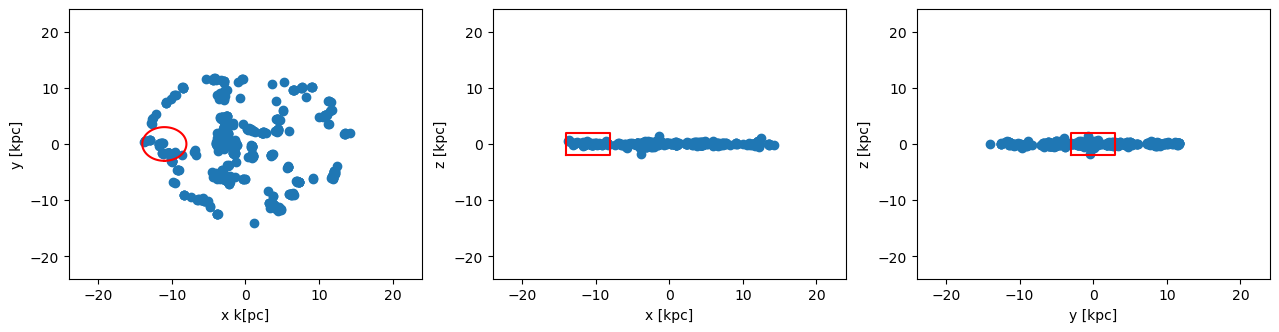

Cylindrical Region: Cutout the data assigned to the object `clumps`

Select the ranges of the cylinder in the unit "kpc", relative to the given center [13., 24., 24.]. The height refers to both z-directions from the plane.

clumps_subregion = subregion( clumps, :cylinder,
                                radius=3.,
                                height=2.,
                                range_unit=:kpc,
                                center=[(24. -11.), :bc, :bc]); # direction=:z, by default

[Mera]: 2026-06-01T20:14:07.602
center: [0.2708333, 0.5, 0.5] ==> [13.0 [kpc] :: 24.0 [kpc] :: 24.0 [kpc]]
domain:
xmin::xmax: 0.2083333 :: 0.3333333  	==> 10.0 [kpc] :: 16.0 [kpc]
ymin::ymax: 0.4375 :: 0.5625  	==> 21.0 [kpc] :: 27.0 [kpc]
zmin::zmax: 0.4583333 :: 0.5416667  	==> 22.0 [kpc] :: 26.0 [kpc]
Radius: 3.0 [kpc]
Height: 2.0 [kpc]
Memory used for data table :5.05078125 KB
-------------------------------------------------------

Extract the the clump positions of the subregion and the extent of the full box:

x, y, z    = getpositions(clumps_subregion, :kpc, center=[:boxcenter])
rx, ry, rz = getextent(clumps, :kpc, center=[:boxcenter]);

figure(figsize=(15.5, 3.5))
theta = range(-pi, stop=pi, length=100)

subplot(1,3,1)
scatter(x,y)
plot( 3. .* sin.(theta) .-11, 3 .* cos.(theta), color="red")
xlim(rx)
ylim(ry)
xlabel("x k[pc]")
ylabel("y [kpc]")

subplot(1,3,2)
scatter(x,z)
plot([-3.,3.,3.,-3.,-3.] .-11.,[-2.,-2.,2.,2.,-2.], color="red")
xlim(rx)
ylim(rz)
xlabel("x [kpc]")
ylabel("z [kpc]")

subplot(1,3,3)
scatter(y,z)
plot([-3.,3.,3.,-3.,-3.],[-2.,-2.,2.,2.,-2.], color="red")
xlim(ry)
ylim(rz)
xlabel("y [kpc]")
ylabel("z [kpc]");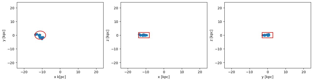

Cylindrical Region: Scatter-Plot of the selected data range with respect to the center of the sub-region:

x, y, z    = getpositions(clumps_subregion, :kpc,
                            center=[ (24. -11.), :bc, :bc],
                            center_unit=:kpc);
rx_sub, ry_sub, rz_sub = getextent(clumps_subregion, :kpc,
                                    center=[ (24. -11.), :bc, :bc],
                                    center_unit=:kpc);

figure(figsize=(15.5, 3.5))
theta = range(-pi, stop=pi, length=100)

subplot(1,3,1)
scatter(x,y)
plot( 3. .* sin.(theta), 3 .* cos.(theta), color="red")
xlim(rx_sub)
ylim(ry_sub)
xlabel("kpc")
ylabel("kpc")

subplot(1,3,2)
scatter(x,z)
xlim(rx_sub)
ylim(rz_sub)
xlabel("kpc")
ylabel("kpc")

subplot(1,3,3)
scatter(y,z)
xlim(ry_sub)
ylim(rz_sub)
xlabel("kpc")
ylabel("kpc");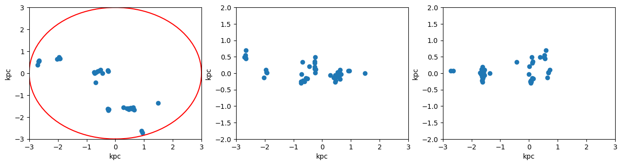

Cylindrical Region: Get the data outside of the selected region (inverse selection):

clumps_subregion = subregion( clumps, :cylinder,
                            radius=3.,
                            height=2.,
                            range_unit=:kpc,
                            center=[ (24. -11.),:bc,:bc],
                            inverse=true);

[Mera]: 2026-06-01T20:14:08.928
center: [0.2708333, 0.5, 0.5] ==> [13.0 [kpc] :: 24.0 [kpc] :: 24.0 [kpc]]
domain:
xmin::xmax: 0.2083333 :: 0.3333333  	==> 10.0 [kpc] :: 16.0 [kpc]
ymin::ymax: 0.4375 :: 0.5625  	==> 21.0 [kpc] :: 27.0 [kpc]
zmin::zmax: 0.4583333 :: 0.5416667  	==> 22.0 [kpc] :: 26.0 [kpc]
Radius: 3.0 [kpc]
Height: 2.0 [kpc]
Memory used for data table :57.73828125
 KB
-------------------------------------------------------

x, y, z    = getpositions(clumps_subregion, :kpc, center=[:boxcenter]);
rx_sub, ry_sub, rz_sub = getextent(clumps_subregion, :kpc, center=[:boxcenter]);

figure(figsize=(15.5, 3.5))
theta = range(-pi, stop=pi, length=100)

subplot(1,3,1)
scatter(x,y)
plot( 3. .* sin.(theta) .-11, 3 .* cos.(theta), color="red")
xlim(rx)
ylim(ry)
xlabel("x k[pc]")
ylabel("y [kpc]")

subplot(1,3,2)
scatter(x,z)
plot([-3.,3.,3.,-3.,-3.] .-11.,[-2.,-2.,2.,2.,-2.], color="red")
xlim(rx)
ylim(rz)
xlabel("x [kpc]")
ylabel("z [kpc]")

subplot(1,3,3)
scatter(y,z)
plot([-3.,3.,3.,-3.,-3.],[-2.,-2.,2.,2.,-2.], color="red")
xlim(ry)
ylim(rz)
xlabel("y [kpc]")
ylabel("z [kpc]");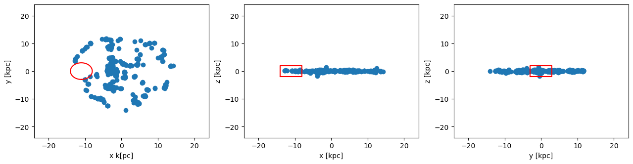

Spherical Region Selection

Spherical selections excel at analyzing centrally concentrated structures, bound systems, or radially distributed phenomena. This isotropic geometric filter is ideal for studying galaxy halos, star-forming regions, or any system with spherical symmetry around a central point.

Key Features:

Radial symmetry - Perfect for centrally concentrated or bound systems
Single parameter control - Specify only radius for complete region definition
Flexible center positioning - Place sphere anywhere in simulation domain
Natural for bound objects - Ideal for analyzing gravitationally bound structures
Scalable analysis - Easy to vary radius for multi-scale investigations

Extract the the clump positions and the extent of the full box:

clumps  = getclumps(info);
x, y, z = getpositions(clumps, :kpc, center=[:boxcenter]);
rx, ry, rz = getextent(clumps, :kpc, center=[:boxcenter]);

[Mera]: Get clump data: 2026-06-01T20:14:09.488
domain:
xmin::xmax: 0.0 :: 1.0  	==> 0.0 [kpc] :: 48.0 [kpc]
ymin::ymax: 0.0 :: 1.0  	==> 0.0 [kpc] :: 48.0 [kpc]
zmin::zmax: 0.0 :: 1.0  	==> 0.0 [kpc] :: 48.0 [kpc]
Read 12 colums:
[:index, :lev, :parent, :ncell, :peak_x, :peak_y, :peak_z, Symbol("rho-"), Symbol("rho+"), :rho_av, :mass_cl, :relevance]
Memory used for data table :
61.58203125 KB
-------------------------------------------------------

The red lines show the region that we want to cut-out as a sub-region from the full data:

figure(figsize=(15.5, 3.5))

theta = range(-pi, stop=pi, length=100)

subplot(1,3,1)
scatter(x,y)
plot( 10. .* sin.(theta) .-11., 10 .* cos.(theta), color="red")
xlim(rx)
ylim(ry)
xlabel("x [kpc]")
ylabel("y [kpc]")

subplot(1,3,2)
scatter(x,z)
plot( 10. .* sin.(theta) .-11., 10 .* cos.(theta), color="red")
xlim(rx)
ylim(rz)
xlabel("x [kpc]")
ylabel("z [kpc]")

subplot(1,3,3)
scatter(y,z)
plot( 10. .* sin.(theta) , 10 .* cos.(theta), color="red")
xlim(ry)
ylim(rz)
xlabel("y [kpc]")
ylabel("z [kpc]")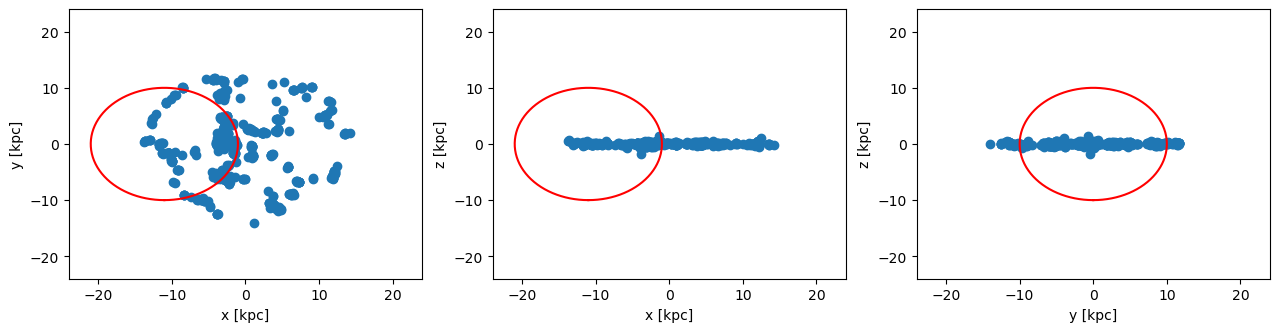

PyObject Text(2615.8235294117653, 0.5, 'z [kpc]')

Spherical Region: Cutout the data assigned to the object `clumps`

Select the radius of the sphere in the unit "kpc", relative to the given center [13., 24., 24.]:

clumps_subregion = subregion( clumps, :sphere,
                                     radius=10.,
                                     range_unit=:kpc,
                                     center=[ (24. -11.),:bc, :bc]);

[Mera]: 2026-06-01T20:14:09.937
center: [0.2708333, 0.5, 0.5] ==> [13.0 [kpc] :: 24.0 [kpc] :: 24.0 [kpc]]
domain:
xmin::xmax: 0.0625 :: 0.4791667  	==> 3.0 [kpc] :: 23.0 [kpc]
ymin::ymax: 0.2916667 :: 0.7083333  	==> 14.0 [kpc] :: 34.0 [kpc]
zmin::zmax: 0.2916667 :: 0.7083333  	==> 14.0 [kpc] :: 34.0 [kpc]
Radius: 10.0 [kpc]
Memory used for data table :28.48828125
 KB
-------------------------------------------------------

x, y, z    = getpositions(clumps_subregion, :kpc, center=[:boxcenter]); # subregion
rx, ry, rz = getextent(clumps, :kpc, center=[:boxcenter]); # full box

figure(figsize=(15.5, 3.5))

theta = range(-pi, stop=pi, length=100)

subplot(1,3,1)
scatter(x,y)
plot( 10. .* sin.(theta) .-11., 10 .* cos.(theta), color="red")
xlim(rx)
ylim(ry)
xlabel("x [kpc]")
ylabel("y [kpc]")

subplot(1,3,2)
scatter(x,z)
plot( 10. .* sin.(theta) .-11., 10 .* cos.(theta), color="red")
xlim(rx)
ylim(rz)
xlabel("x [kpc]")
ylabel("z [kpc]")

subplot(1,3,3)
scatter(y,z)
plot( 10. .* sin.(theta) , 10 .* cos.(theta), color="red")
xlim(ry)
ylim(rz)
xlabel("y [kpc]")
ylabel("z [kpc]");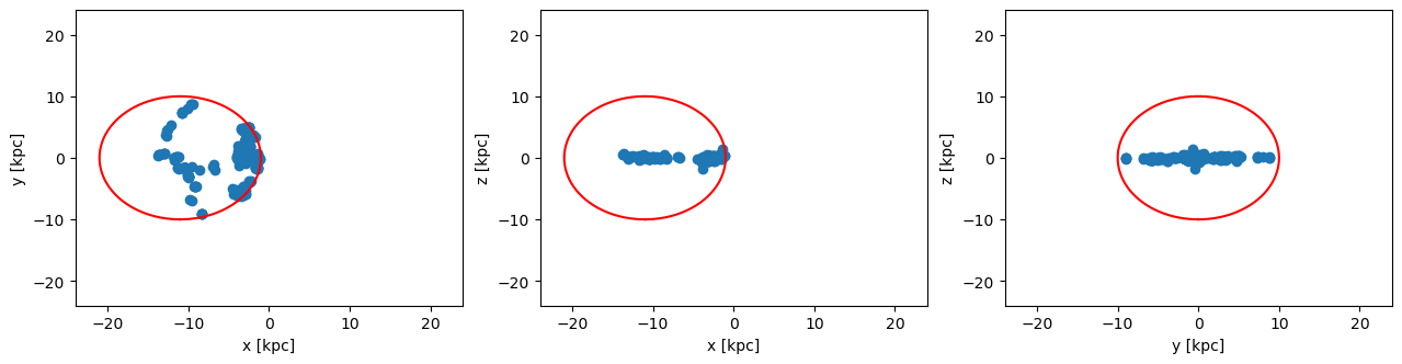

Spherical Region: Scatter-Plot of the selected data range with respect to the center of the sub-region:

x, y, z    = getpositions(clumps_subregion, :kpc,
                            center=[ (24. -11.), :bc, :bc],
                            center_unit=:kpc); # subregion
rx_sub, ry_sub, rz_sub = getextent(clumps_subregion, :kpc,
                            center=[(24. -11.), :bc, :bc],
                            center_unit=:kpc); # subregion

figure(figsize=(15.5, 3.5))
theta = range(-pi, stop=pi, length=100)

subplot(1,3,1)
scatter(x,y)
plot( 10. .* sin.(theta), 10 .* cos.(theta), color="red")
xlim(rx_sub)
ylim(ry_sub)
xlabel("x [kpc]")
ylabel("y [kpc]")

subplot(1,3,2)
scatter(x,z)
plot( 10. .* sin.(theta), 10 .* cos.(theta), color="red")
xlim(rx_sub)
ylim(rz_sub)
xlabel("x [kpc]")
ylabel("z [kpc]")

subplot(1,3,3)
scatter(y,z)
plot( 10. .* sin.(theta), 10 .* cos.(theta), color="red")
xlim(ry_sub)
ylim(rz_sub)
xlabel("y [kpc]")
ylabel("z [kpc]");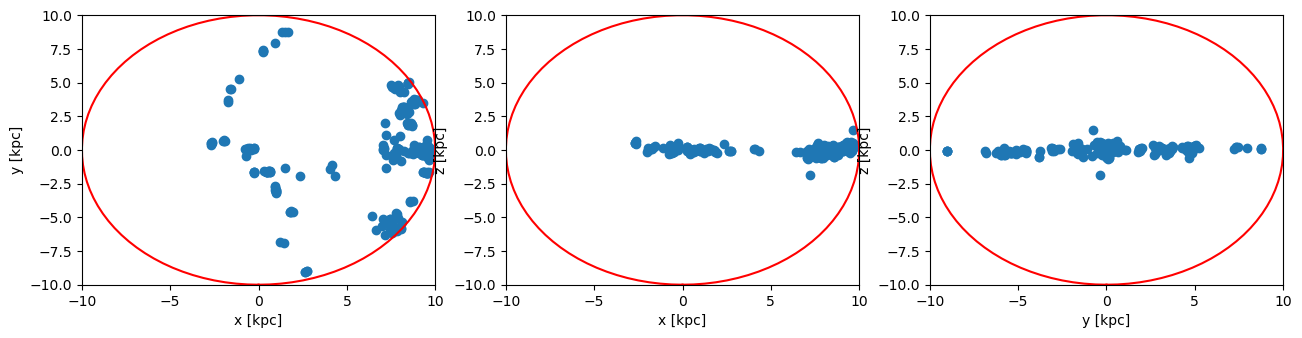

Spherical Region: Get the data outside of the selected region (inverse selection):

clumps_subregion = subregion( clumps, :sphere,
                                     radius=10.,
                                     range_unit=:kpc,
                                     center=[ (24. -11.),:bc,:bc],
                                     inverse=true);

[Mera]: 2026-06-01T20:14:10.469
center: [0.2708333, 0.5, 0.5] ==> [13.0 [kpc] :: 24.0 [kpc] :: 24.0 [kpc]]
domain:
xmin::xmax: 0.0625 :: 0.4791667  	==> 3.0 [kpc] :: 23.0 [kpc]
ymin::ymax: 0.2916667 :: 0.7083333  	==> 14.0 [kpc] :: 34.0 [kpc]
zmin::zmax: 0.2916667 :: 0.7083333  	==> 14.0 [kpc] :: 34.0 [kpc]
Radius: 10.0 [kpc]
Memory used for data table :34.30078125 KB
-------------------------------------------------------

x, y, z    = getpositions(clumps_subregion, :kpc, center=[:boxcenter]);
rx_sub, ry_sub, rz_sub = getextent(clumps_subregion, :kpc, center=[:boxcenter]);

figure(figsize=(15.5, 3.5))

theta = range(-pi, stop=pi, length=100)

subplot(1,3,1)
scatter(x,y)
plot( 10. .* sin.(theta) .-11., 10 .* cos.(theta), color="red")
xlim(rx)
ylim(ry)
xlabel("x [kpc]")
ylabel("y [kpc]")

subplot(1,3,2)
scatter(x,z)
plot( 10. .* sin.(theta) .-11., 10 .* cos.(theta), color="red")
xlim(rx)
ylim(rz)
xlabel("x [kpc]")
ylabel("z [kpc]")

subplot(1,3,3)
scatter(y,z)
plot( 10. .* sin.(theta) , 10 .* cos.(theta), color="red")
xlim(ry)
ylim(rz)
xlabel("y [kpc]")
ylabel("z [kpc]")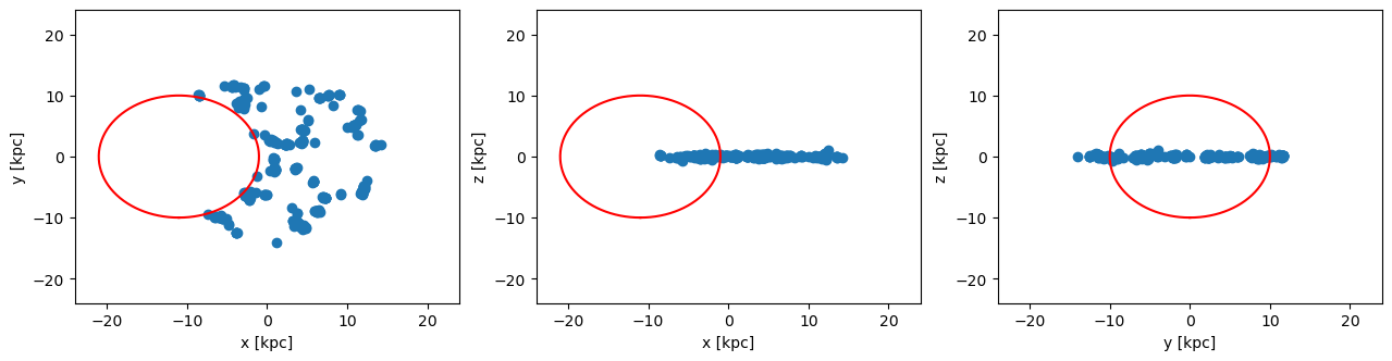

PyObject Text(2615.8235294117653, 0.5, 'z [kpc]')

Advanced Selection Techniques

Combined and Nested Regions

The spatial selection functions in MERA offer powerful composition capabilities, allowing you to create complex selection criteria by combining multiple geometric filters. This enables sophisticated analysis of irregular structures or multi-component systems.

Key Composition Features:

Sequential application - Apply multiple filters in sequence for intersection operations
Nested selections - Create hierarchical spatial selections with different scales
Overlapping regions - Analyze overlapping spatial domains simultaneously
Boolean operations - Combine regions with AND/OR logic through successive filtering

Practical Applications:

Multi-scale analysis - Study structures at different resolution scales
Complex geometries - Approximate irregular shapes with geometric combinations
Comparative studies - Analyze multiple regions with consistent methodologies
Hierarchical systems - Study parent-child relationships in clump hierarchies

The sub-region functions can be used in any combination with each other! (Combined with overlapping ranges or nested)

Cylindrical Shell Selection

Cylindrical shells provide specialized tools for analyzing hollow cylindrical structures, disk-like systems with central cavities, or annular regions in rotating systems. This geometry is particularly valuable for studying galactic disks, accretion disk structures, or jet boundaries.

Key Features:

Hollow geometry - Excludes central cylindrical region for annular analysis
Inner/outer radius control - Precise specification of shell thickness
Height specification - Define cylindrical extent along rotation axis
Directional flexibility - Orient cylinder axis along any coordinate direction
Perfect for disk systems - Ideal for analyzing galactic disk structures or rotating media

Shell Region Applications:

Disk galaxy analysis - Study stellar disk structure excluding central bulge
Accretion disk features - Analyze disk material while avoiding central object
Jet boundary studies - Examine material around jet axes
Ring structure analysis - Investigate annular features in rotating systems

Extract the the clump positions and the extent of the full box:

clumps = getclumps(info);
x, y, z = getpositions(clumps, :kpc, center=[:boxcenter]);
rx, ry, rz = getextent(clumps, :kpc, center=[:boxcenter]);

[Mera]: Get clump data: 2026-06-01T20:14:10.732
domain:
xmin::xmax: 0.0 :: 1.0  	==> 0.0 [kpc] :: 48.0 [kpc]
ymin::ymax: 0.0 :: 1.0  	==> 0.0 [kpc] :: 48.0 [kpc]
zmin::zmax: 0.0 :: 1.0  	==> 0.0 [kpc] :: 48.0 [kpc]
Read 12 colums:
[:index, :lev, :parent, :ncell, :peak_x, :peak_y, :peak_z, Symbol("rho-"), Symbol("rho+"), :rho_av, :mass_cl, :relevance]
Memory used for data table :61.58203125 KB
-------------------------------------------------------

The red lines show the shell that we want to cut-out as a sub-region from the full data:

figure(figsize=(15.5, 3.5))
theta = range(-pi, stop=pi, length=100)

subplot(1,3,1)
scatter(x,y)
plot( 10. .* sin.(theta) , 10 .* cos.(theta), color="red")
plot( 5. .* sin.(theta) , 5. .* cos.(theta), color="red", ls="--")
xlim(rx)
ylim(ry)
xlabel("x k[pc]")
ylabel("y [kpc]")

subplot(1,3,2)
scatter(x,z)
plot([-10.,-10.,10.,10.,-10.], [-2.,2.,2.,-2.,-2.], color="red")
plot([-5.,-5,5.,5.,-5.], [-2.,2.,2.,-2.,-2.], color="red", ls="--")
xlim(rx)
ylim(rz)
xlabel("x [kpc]")
ylabel("z [kpc]")

subplot(1,3,3)
scatter(y,z)
plot([-10.,-10.,10.,10.,-10.], [-2.,2.,2.,-2.,-2.], color="red")
plot([-5.,-5,5.,5.,-5.], [-2.,2.,2.,-2.,-2.], color="red",ls = "--")
xlim(ry)
ylim(rz)
xlabel("y [kpc]")
ylabel("z [kpc]");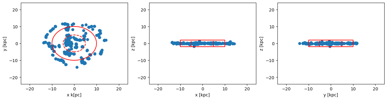

Cylindrical Shell:

Pass the height of the cylinder and the inner/outer radius of the shell in the unit "kpc", relative to the box center [24., 24., 24.]:

clumps_subregion = shellregion( clumps, :cylinder,
                                         radius=[5.,10.],
                                         height=2.,
                                         range_unit=:kpc,
                                         center=[:boxcenter]);

[Mera]: 2026-06-01T20:14:11.250
center: [0.5, 0.5, 0.5] ==> [24.0 [kpc] :: 24.0 [kpc] :: 24.0 [kpc]]
domain:
xmin::xmax: 0.2916667 :: 0.7083333  	==> 14.0 [kpc] :: 34.0 [kpc]
ymin::ymax: 0.2916667 :: 0.7083333  	==> 14.0 [kpc] :: 34.0 [kpc]
zmin::zmax: 0.4583333 :: 0.5416667  	==> 22.0 [kpc] :: 26.0 [kpc]
Inner radius: 5.0 [kpc]
Outer radius: 10.0 [kpc]
Radius diff: 5.0 [kpc]
Height: 2.0 [kpc]
Memory used for data table :18.36328125 KB
-------------------------------------------------------

x, y, z    = getpositions(clumps_subregion, :kpc, center=[:boxcenter]); # shellregion
rx, ry, rz = getextent(clumps, :kpc, center=[:boxcenter]); # full box

figure(figsize=(15.5, 3.5))
theta = range(-pi, stop=pi, length=100)

subplot(1,3,1)
scatter(x,y)
plot( 10. .* sin.(theta) , 10 .* cos.(theta), color="red")
plot( 5. .* sin.(theta) , 5. .* cos.(theta), color="red", ls="--")
xlim(rx)
ylim(ry)
xlabel("x k[pc]")
ylabel("y [kpc]")

subplot(1,3,2)
scatter(x,z)
plot([-10.,-10.,10.,10.,-10.], [-2.,2.,2.,-2.,-2.], color="red")
plot([-5.,-5,5.,5.,-5.], [-2.,2.,2.,-2.,-2.], color="red", ls="--")
xlim(rx)
ylim(rz)
xlabel("x [kpc]")
ylabel("z [kpc]")

subplot(1,3,3)
scatter(y,z)
plot([-10.,-10.,10.,10.,-10.], [-2.,2.,2.,-2.,-2.], color="red")
plot([-5.,-5,5.,5.,-5.], [-2.,2.,2.,-2.,-2.], color="red", ls="--")
xlim(ry)
ylim(rz)
xlabel("y [kpc]")
ylabel("z [kpc]");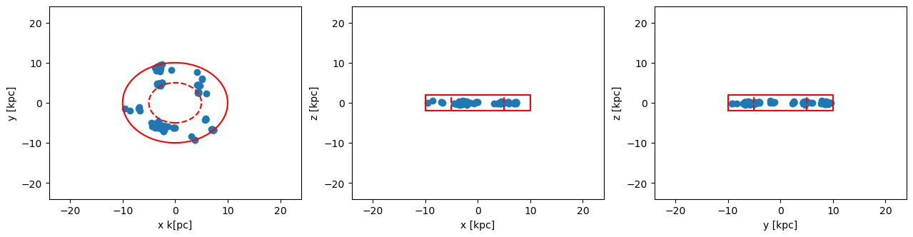

Cylindrical Shell: Get the data outside of the selected shell-region (inverse selection):

clumps_subregion = shellregion( clumps, :cylinder,
                                         radius=[5.,10.],
                                         height=2.,
                                         range_unit=:kpc,
                                         center=[:boxcenter],
                                         inverse=true);

[Mera]: 2026-06-01T20:14:11.544
center: [0.5, 0.5, 0.5] ==> [24.0 [kpc] :: 24.0 [kpc] :: 24.0 [kpc]]
domain:
xmin::xmax: 0.2916667 :: 0.7083333  	==> 14.0 [kpc] :: 34.0 [kpc]
ymin::ymax: 0.2916667 :: 0.7083333  	==> 14.0 [kpc] :: 34.0 [kpc]
zmin::zmax: 0.4583333 :: 0.5416667  	==> 22.0 [kpc] :: 26.0 [kpc]
Inner radius: 5.0 [kpc]
Outer radius: 10.0 [kpc]
Radius diff: 5.0 [kpc]
Height: 2.0 [kpc]
Memory used for data table :44.42578125 KB
-------------------------------------------------------

x, y, z    = getpositions(clumps_subregion, :kpc, center=[:boxcenter]); # shellregion
rx, ry, rz = getextent(clumps, :kpc, center=[:boxcenter]); # full box

figure(figsize=(15.5, 3.5))
theta = range(-pi, stop=pi, length=100)

subplot(1,3,1)
scatter(x,y)
plot( 10. .* sin.(theta) , 10 .* cos.(theta), color="red")
plot( 5. .* sin.(theta) , 5. .* cos.(theta), color="red", ls="--")
xlim(rx)
ylim(ry)
xlabel("x k[pc]")
ylabel("y [kpc]")

subplot(1,3,2)
scatter(x,z)
plot([-10.,-10.,10.,10.,-10.], [-2.,2.,2.,-2.,-2.], color="red")
plot([-5.,-5,5.,5.,-5.], [-2.,2.,2.,-2.,-2.], color="red", ls="--")
xlim(rx)
ylim(rz)
xlabel("x [kpc]")
ylabel("z [kpc]")

subplot(1,3,3)
scatter(y,z)
plot([-10.,-10.,10.,10.,-10.], [-2.,2.,2.,-2.,-2.], color="red")
plot([-5.,-5,5.,5.,-5.], [-2.,2.,2.,-2.,-2.], color="red", ls="--")
xlim(ry)
ylim(rz)
xlabel("y [kpc]")
ylabel("z [kpc]");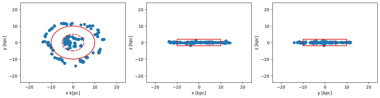

Spherical Shell

Extract the the clump positions and the extent of the full box:

clumps  = getclumps(info);
x, y, z = getpositions(clumps, :kpc, center=[:boxcenter]);
rx, ry, rz = getextent(clumps, :kpc, center=[:boxcenter]);

[Mera]: Get clump data: 2026-06-01T20:14:11.878
domain:
xmin::xmax: 0.0 :: 1.0  	==> 0.0 [kpc] :: 48.0 [kpc]
ymin::ymax: 0.0 :: 1.0  	==> 0.0 [kpc] :: 48.0 [kpc]
zmin::zmax: 0.0 :: 1.0  	==> 0.0 [kpc] :: 48.0 [kpc]
Read 12 colums:
[:index, :lev, :parent, :ncell, :peak_x, :peak_y, :peak_z, Symbol("rho-"), Symbol("rho+"), :rho_av, :mass_cl, :relevance]
Memory used for data table :
61.58203125 KB
-------------------------------------------------------

The red lines show the shell that we want to cut-out as a sub-region from the full data:

figure(figsize=(15.5, 3.5))
theta = range(-pi, stop=pi, length=100)

subplot(1,3,1)
scatter(x,y)
plot( 10. .* sin.(theta) , 10 .* cos.(theta), color="red")
plot( 5. .* sin.(theta) , 5. .* cos.(theta), color="red", ls="--")
xlim(rx)
ylim(ry)
xlabel("x k[pc]")
ylabel("y [kpc]")

subplot(1,3,2)
scatter(x,z)
plot( 10. .* sin.(theta) , 10 .* cos.(theta), color="red")
plot( 5. .* sin.(theta) , 5. .* cos.(theta), color="red", ls="--")
xlim(rx)
ylim(rz)
xlabel("x [kpc]")
ylabel("z [kpc]")

subplot(1,3,3)
scatter(y,z)
plot( 10. .* sin.(theta) , 10 .* cos.(theta), color="red")
plot( 5. .* sin.(theta) , 5. .* cos.(theta), color="red", ls="--")
xlim(ry)
ylim(rz)
xlabel("y [kpc]")
ylabel("z [kpc]");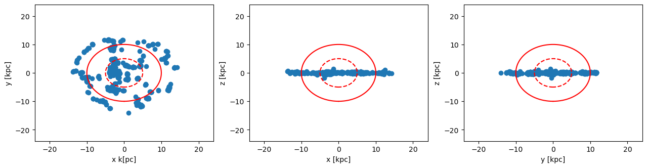

Spherical Shell:

Select the inner and outer radius of the spherical shell in unit "kpc", relative to the box center [24., 24., 24.]:

clumps_subregion = shellregion( clumps, :sphere,
                                radius=[5.,10.],
                                range_unit=:kpc,
                                center=[:boxcenter]);

[Mera]: 2026-06-01T20:14:12.986
center: [0.5, 0.5, 0.5] ==> [24.0 [kpc] :: 24.0 [kpc] :: 24.0 [kpc]]
domain:
xmin::xmax: 0.2916667 :: 0.7083333  	==> 14.0 [kpc] :: 34.0 [kpc]
ymin::ymax: 0.2916667 :: 0.7083333  	==> 14.0 [kpc] :: 34.0 [kpc]
zmin::zmax: 0.2916667 :: 0.7083333  	==> 14.0 [kpc] :: 34.0 [kpc]
Inner radius: 5.0 [kpc]
Outer radius: 10.0 [kpc]
Radius diff: 5.0 [kpc]
Memory used for data table :18.36328125 KB
-------------------------------------------------------

x, y, z    = getpositions(clumps_subregion, :kpc, center=[:boxcenter]); # shellregion
rx, ry, rz = getextent(clumps, :kpc, center=[:boxcenter]); # full box

figure(figsize=(15.5, 3.5))
theta = range(-pi, stop=pi, length=100)

subplot(1,3,1)
scatter(x,y)
plot( 10. .* sin.(theta) , 10 .* cos.(theta), color="red")
plot( 5. .* sin.(theta) , 5. .* cos.(theta), color="red", ls="--")
xlim(rx)
ylim(ry)
xlabel("x k[pc]")
ylabel("y [kpc]")

subplot(1,3,2)
scatter(x,z)
plot( 10. .* sin.(theta) , 10 .* cos.(theta), color="red")
plot( 5. .* sin.(theta) , 5. .* cos.(theta), color="red", ls="--")
xlim(rx)
ylim(rz)
xlabel("x [kpc]")
ylabel("z [kpc]")

subplot(1,3,3)
scatter(y,z)
plot( 10. .* sin.(theta) , 10 .* cos.(theta), color="red")
plot( 5. .* sin.(theta) , 5. .* cos.(theta), color="red",  ls="--")
xlim(ry)
ylim(rz)
xlabel("y [kpc]")
ylabel("z [kpc]");

Spherical Shell: Get the data outside of the selected shell-region (inverse selection):

clumps_subregion = shellregion( clumps, :sphere,
                                radius=[5.,10.],
                                range_unit=:kpc,
                                center=[:boxcenter],
                                inverse=true);

[Mera]: 2026-06-01T20:14:13.344
center: [0.5, 0.5, 0.5] ==> [24.0 [kpc] :: 24.0 [kpc] :: 24.0 [kpc]]
domain:
xmin::xmax: 0.2916667 :: 0.7083333  	==> 14.0 [kpc] :: 34.0 [kpc]
ymin::ymax: 0.2916667 :: 0.7083333  	==> 14.0 [kpc] :: 34.0 [kpc]
zmin::zmax: 0.2916667 :: 0.7083333  	==> 14.0 [kpc] :: 34.0 [kpc]
Inner radius: 5.0 [kpc]
Outer radius: 10.0 [kpc]
Radius diff: 5.0 [kpc]
Memory used for data table :44.42578125 KB
-------------------------------------------------------

x, y, z    = getpositions(clumps_subregion, :kpc, center=[:boxcenter]); # shellregion
rx, ry, rz = getextent(clumps, :kpc, center=[:boxcenter] ); # full box

figure(figsize=(15.5, 3.5))
theta = range(-pi, stop=pi, length=100)

subplot(1,3,1)
scatter(x,y)
plot( 10. .* sin.(theta) , 10 .* cos.(theta), color="red")
plot( 5. .* sin.(theta) , 5. .* cos.(theta), color="red", ls="--")
xlim(rx)
ylim(ry)
xlabel("x k[pc]")
ylabel("y [kpc]")

subplot(1,3,2)
scatter(x,z)
plot( 10. .* sin.(theta) , 10 .* cos.(theta), color="red")
plot( 5. .* sin.(theta) , 5. .* cos.(theta), color="red", ls="--")
xlim(rx)
ylim(rz)
xlabel("x [kpc]")
ylabel("z [kpc]")

subplot(1,3,3)
scatter(y,z)
plot( 10. .* sin.(theta) , 10 .* cos.(theta), color="red")
plot( 5. .* sin.(theta) , 5. .* cos.(theta), color="red", ls="--")
xlim(ry)
ylim(rz)
xlabel("y [kpc]")
ylabel("z [kpc]");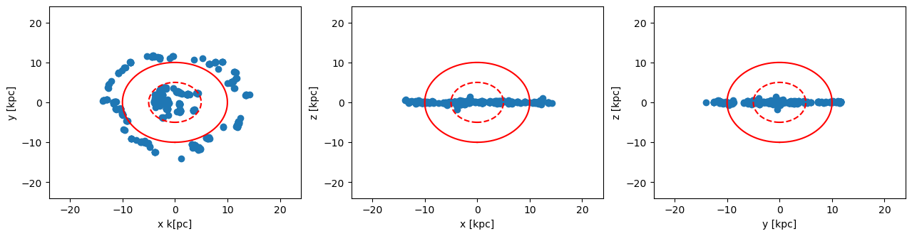

Value-Type Regions

subregion also accepts composable region value types — Sphere, Cuboid, Cylinder, SphericalShell — that compose with the boolean operators ∩ ∪ \ !. Clumps are points (their peak position), so the region is a point-membership test; inverse=true selects the complement.

# clumps inside a ball about the box centre, and the complement
clumps_in  = subregion(clumps, Sphere(20.0; center=[:bc], range_unit=:kpc))
clumps_out = subregion(clumps, Sphere(20.0; center=[:bc], range_unit=:kpc), inverse=true)
println("inside: ", length(clumps_in.data), "   outside: ", length(clumps_out.data),
        "   total: ", length(clumps.data))
x, y, z = getpositions(clumps_in, :kpc, center=[:boxcenter]);

inside: 644   outside: 0   total: 644

Boolean Combinations

Build composite selections — e.g. a ball with a central cylinder removed:

clumps_sel = subregion(clumps, Sphere(30.0; range_unit=:kpc) \ Cylinder(8.0, 30.0; range_unit=:kpc))
println("type: ", typeof(clumps_sel), "   selected clumps: ", length(clumps_sel.data))

type: ClumpDataType   selected clumps: 292

Shell Regions

clumps_shell = subregion(clumps, SphericalShell(5.0, 20.0; range_unit=:kpc))
println("clumps in spherical shell [5,20] kpc: ", length(clumps_shell.data), " / ", length(clumps.data))

clumps in spherical shell [5,20] kpc: 427 / 644

Summary

Key Techniques Mastered

Through this comprehensive tutorial, you have gained expertise in advanced spatial selection techniques for clump analysis:

Geometric Selection Methods:

Cuboid regions - Rectangular box selections with independent axis control
Cylindrical regions - Axially symmetric selections for rotating systems
Spherical regions - Radially symmetric selections for bound structures
Shell regions - Hollow geometric selections with inner/outer boundaries

Advanced Capabilities:

Inverse selections - Extract data outside specified regions
Combined filters - Sequential application for complex geometries
Unit conversion - Seamless work with physical units (kpc, Mpc, etc.)
Center references - Flexible coordinate system positioning

Coordinate System Flexibility:

Standard notation [0:1] - Normalized simulation coordinates
Physical units - Real astronomical distances with automatic conversion
Custom centers - User-defined reference points for analysis
Box-centered shortcuts - Convenient :boxcenter positioning

Practical Applications

These spatial selection techniques enable sophisticated clump analysis workflows:

Scientific Use Cases:

Hierarchical analysis - Study clump structures at multiple scales
Environmental studies - Analyze clump properties in different regions
Evolutionary tracking - Follow clump development in specific volumes
Comparative analysis - Contrast clump populations across regions

Analysis Workflows:

Multi-scale investigations - Combine different geometric selections
Statistical studies - Generate clean samples for population analysis
Visualization preparation - Extract regions for focused plotting
Data reduction - Manage memory by selecting relevant subsets

Performance Considerations

Memory Management:

Use spatial selections to reduce memory footprint for large simulations
Apply filters early in analysis pipeline to optimize performance
Combine geometric selections efficiently to minimize data processing

Computational Efficiency:

Leverage inverse selections for excluding large regions
Use appropriate coordinate systems for your analysis scale
Consider shell regions for hollow structures to reduce data volume

Integration with MERA Ecosystem

These spatial selection techniques integrate seamlessly with other MERA analysis functions:

Compatible Functions:

getpositions() - Extract coordinates with unit conversion
getextent() - Calculate spatial bounds and ranges
dataoverview() - Statistical analysis of selected regions
msum(), mmean() - Statistical calculations on spatial subsets

Workflow Integration:

Combine with loading functions for targeted data acquisition
Chain with analysis functions for comprehensive studies
Link with visualization tools for publication-quality figures