Statistics: PDFs

pdf computes the probability distribution function of any getvar quantity over the cells (or particles) of a snapshot. The canonical use is the density PDF — the log-normal core (with a power-law high-density tail) that supersonic turbulence and self-gravity imprint on the gas, and the starting point for many star-formation models.

using Mera
gas = gethydro(getinfo(100, "/data/Mera-Tests/spiral_clumps"))

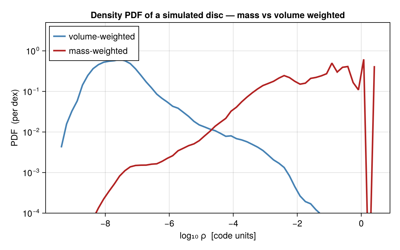
P  = pdf(gas, :rho)                    # mass-weighted density PDF
Pv = pdf(gas, :rho; weight=:volume)    # volume-weighted

# plot, e.g.
# lines(log10.(P.centers), P.pdf)

What it returns

pdf returns a NamedTuple (centers, edges, pdf, logbins, quantity, unit, weight):

• centers / edges — bin centres / edges, in the quantity's units.

• pdf — a probability density on the binning axis. With logbins=true (the default) the axis is log10(quantity), so pdf is a density per dex; with logbins=false it is a density per unit. Either way it is normalised to unit area:

  sum(P.pdf .* diff(log10.(P.edges))) ≈ 1     # logbins
  sum(P.pdf .* diff(P.edges)) ≈ 1             # linear bins

Weighting

The weight decides what the PDF describes — and the two weightings tell different stories (as in the figure):

• weight=:mass (default) — "how much mass is at each density"; peaks at high density.
• weight=:volume — "how much volume is at each density"; the volume-weighted density PDF is the one compared with turbulence theory (the log-normal).
• weight=:cells / :count — number-weighted (every cell counts equally).

Options

The norm choices answer different questions: :density is the proper (bin-width-independent) PDF for comparing against theory or different binnings; :probability gives the mass/volume fraction in each bin; :peak compares shapes regardless of amplitude; :count keeps the raw weighted histogram.

It works on any quantity, not just density — e.g. pdf(gas, :T) (temperature), pdf(gas, :mach) (Mach number), pdf(gas, :p) (pressure). Combine with subregion or a mask to restrict to a region, and with timeseries to watch a PDF evolve.

Any data type — and projected 2D maps

pdf is generic over the data object, so it works on hydro, particle, gravity, and RT data — any quantity/weight getvar supports. For a signed field (the potential :epot, a velocity component) pass logbins=false, since log bins need positive values:

pdf(particles, :vx;   weight=:mass,   logbins=false)   # particle velocity PDF
pdf(gravity,   :epot; weight=:volume, logbins=false)   # potential PDF
pdf(rt,        :Np1;  weight=:volume)                  # photon-density PDF

Pass a projection result and pdf takes the PDF of the 2D map's pixels — with :sd this is the column-density PDF (N-PDF), a standard observational diagnostic. Weight by :area (default, every pixel equal), :value, or another map key; a raw matrix works too:

p = projection(gas, :sd)
N = pdf(p, :sd)                                              # area-weighted N-PDF
M = pdf(mock_observe(p, :sd; beam_fwhm=1.0, beam_unit=:kpc)) # PDF of a raw image matrix

Planned

Density/velocity power spectra and structure functions are planned as a follow-up; they need an FFT backend and will ship as a package extension (using FFTW), the same way savefits uses FITSIO. Many derived quantities are already available through getvar — e.g. :freefall_time, :jeanslength/:jeansmass, :virial_parameter_local, the sound speed :cs, and the Mach numbers :mach*.

See also

• getvar — the quantities you can take a PDF of (and the derived timescales).
• profile — radial/quantity profiles (means in bins), the complementary view.
• timeseries — evolve a PDF across snapshots.