Reading PLUTO data (experimental)

Mera's analysis layer is code-blind: it works on a generic uniform/AMR cell list, not on RAMSES file formats. This page adds a frontend for the PLUTO code that reads PLUTO's output into the same Mera structs — so getvar, projection, pdf, timeseries, getmovie and the rest run on PLUTO data unchanged.

Usage

The normal getinfo / gethydro entry points auto-detect PLUTO from its signature files (grid.out + dbl.out) — nothing special to call:

julia> info = getinfo(5, "/data/pluto_sedov3d");   # detects PLUTO

Code: PLUTO
output: 5  time: 0.5 [code units]
grid: 64³ uniform Cartesian, level 6, boxlen = 1.0
variables: (rho, vx, vy, vz, p)
-------------------------------------------------------

julia> gas = gethydro(info);                        # → the PLUTO frontend, code-blind downstream

The overview reports the code, the uniform 64³ grid (mapped to Mera level = log₂64 = 6), the box length and the variable list — the same overview a RAMSES snapshot prints. gas is an ordinary HydroDataType (columns :cx,:cy,:cz, :rho,:vx,:vy,:vz,:p), so the whole analysis layer works:

msum(gas, :Msol); projection(gas, :rho); pdf(gas, :rho)      # the usual calls, unchanged

Force the code with code= (:pluto / :chombo / :ramses / :auto), or call the frontend directly with getinfo_pluto / gethydro_pluto.

Loading a spatial sub-region

gethydro honours the RAMSES spatial-window arguments xrange/yrange/zrange (with center/range_unit), so you load only the part of the box you need:

gas = gethydro(info; xrange=[0.0, 0.5], yrange=[0.25, 0.75], range_unit=:standard)   # a sub-box

The selection acts on the cells, so it is an exact filter and the returned object records the window in gas.ranges; resolution is chosen later at analysis time (projection(…, res=)), not at load.

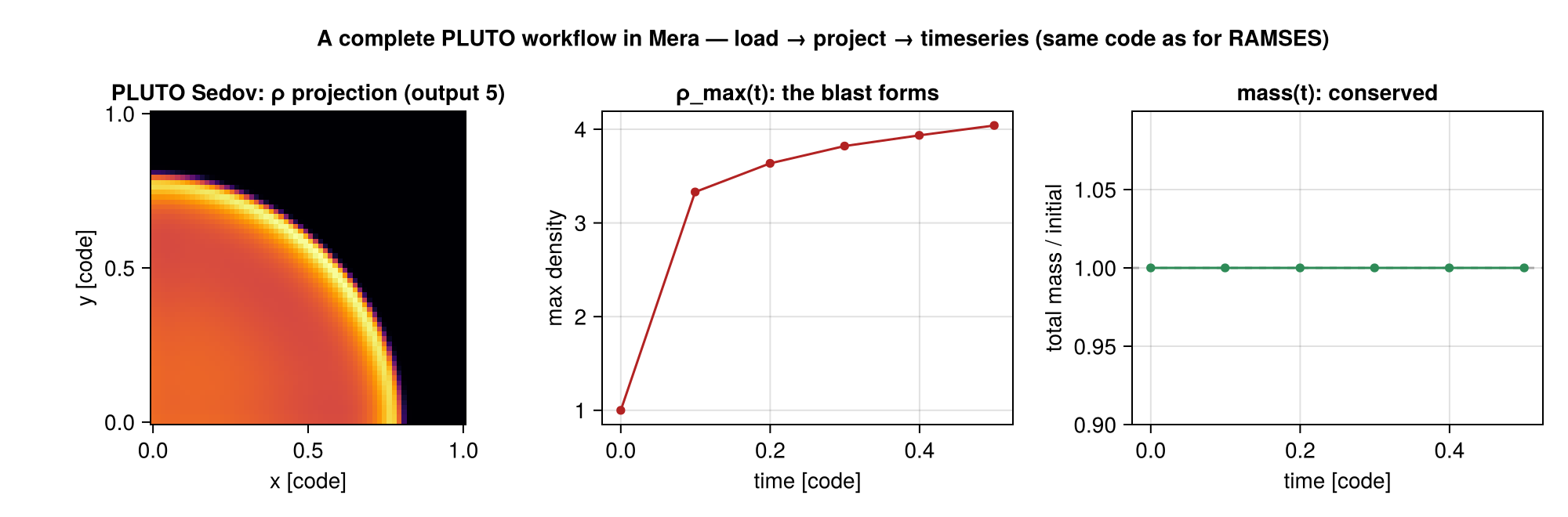
Worked example: the 3-D Sedov blast

Because PLUTO data lands in the standard structs, the entire Mera workflow runs on it — identical to the RAMSES tutorials. Here is load → inspect → projection → time-series → movie → PDF, end to end, on a 3-D Sedov blast (6 PLUTO outputs):

using Mera
path = "/data/pluto_sedov3d"

info = getinfo(5, path); gas = gethydro(info)              # 1. load (auto-detects PLUTO)

extrema(getvar(gas, :rho))                                 # 2. inspect — getvar works unchanged
getvar(gas, :cellsize)[1]                                  #    = boxlen / 2^level
msum(gas)                                                  #    total mass (code units)

p = projection(gas, :sd, res=512, center=[:bc], direction=:z)   # 3. projection (off-axis engine)

ts = timeseries(path, d -> (rho_max = maximum(getvar(d, :rho)), mass = msum(d));   # 4. time series
                time_unit = :standard)                     #    over all 6 outputs (reads dbl.out)

mv = getmovie(path, :rho; time_unit = :standard)           # 5. movie of the blast → GIF
savemovie(mv, "pluto_blast.gif"; tags = :output)

P = pdf(gas, :rho)                                         # 6. density PDF
savemap(p, "pluto_rho.jld2")                               # 7. persist a map (opens in h5py too)

Projecting the loaded blast along each axis shows the spherical shock front directly (the Sedov test runs in one octant, so the shell appears as a quarter-circle from each direction):

using CairoMakie

fig = Figure(size=(1150, 380))
for (i, dir) in enumerate((:x, :y, :z))
    Σ  = projection(gas, :sd, res=512, center=[:bc], direction=dir).maps[:sd]
    ax = Axis(fig[1, i]; title="PLUTO Sedov 3-D — direction :$dir", aspect=DataAspect())
    hidedecorations!(ax)
    heatmap!(ax, log10.(Σ' .+ 1e-30); colormap=:inferno)   # transpose: array (col,row) → (x,y)
end
save("pluto_projection.png", fig, px_per_unit=2)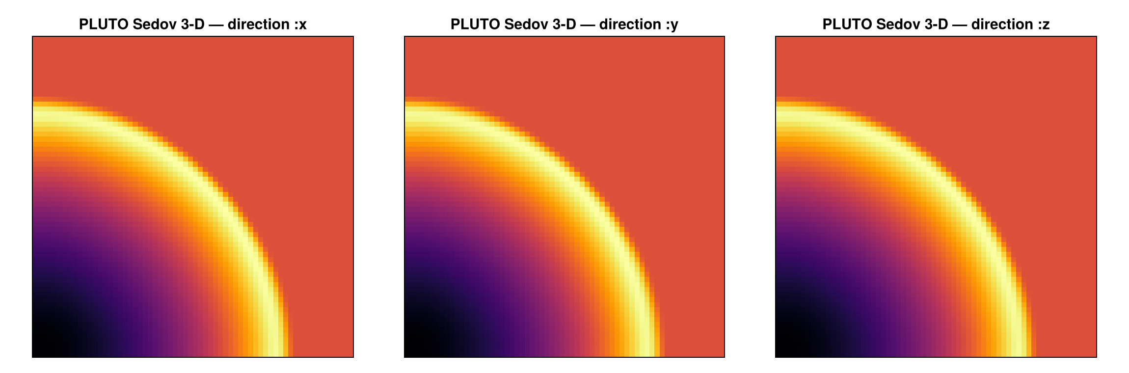

Every step above is the same call you would make on a RAMSES snapshot — that is the whole point of the code-blind analysis layer.

Units

PLUTO writes data in code units and does not store its UNIT_* constants in the output (they live in the run's compiled definitions.h), so by default the run is treated as dimensionless. Pass PLUTO's UNIT_LENGTH/UNIT_DENSITY/UNIT_VELOCITY (in CGS) to make every getvar/projection conversion physical:

# e.g. UNIT_LENGTH = 1 pc, UNIT_DENSITY = m_p, UNIT_VELOCITY = 1 km/s
info = getinfo_pluto(5, path; unit_length=3.086e18, unit_density=1.67e-24, unit_velocity=1e5)
getvar(gethydro(info), :x, :pc)            # now physically correct

Variable names

PLUTO variable names are mapped to Mera's canonical symbols: rho→:rho, vx1/vx2/vx3→:vx/:vy/:vz, prs→:p, and bx1/2/3→:bx/:by/:bz for MHD. Unmapped names pass through as-is.

How it maps onto Mera's grid

The frontend reads PLUTO's static-grid output (the format documented by PLUTO's own pyPLUTO reader):

• grid.out — geometry, per-axis cell count and edges → the cell centres.
• dbl.out — one row per snapshot: time, file mode (single_file), endianness, variable names.
• data.NNNN.dbl — the raw double-precision data (single-file, x1 fastest).

It fills the existing InfoType / HydroDataType (simcode = "PLUTO", levelmin == levelmax, boxlen, the scale, the cell table in the RAMSES convention). The one thing the reader must get exactly right is the cell-coordinate mapping (cell centre = (c − 0.5)·boxlen/2^level); it is validated against pyPLUTO — the density peak and every value match cell-for-cell.

PLUTO particles

If a PLUTO run wrote Lagrangian particles (particles.NNNN.dbl), getinfo flags them and getparticles reads them into a Mera PartDataType, so the particle analysis runs unchanged:

info = getinfo(5, "/data/pluto_run")      # info.particles == true if a particle file is present
part = getparticles(info)                  # → PartDataType (:x,:y,:z, :id, :vx,:vy,:vz, …)
getvar(part, :vx); msum(part)              # the usual particle analysis

The format (an ASCII # header — field_names/field_dim/nparticles/endianity — followed by particle-major binary) is read directly; field names map to Mera symbols (x1→:x, vx1→:vx, …), extra fields keep their names.

PLUTO-AMR (Chombo)

PLUTO's AMR output uses the Chombo box-structured HDF5 format (shared with Orion and other Chombo codes). The frontend reads it too — getinfo auto-detects a .hdf5 snapshot and loads the level hierarchy as a Mera AMR HydroDataType:

info = getinfo(0, "/data/chombo_run")     # detects the Chombo .hdf5 → "Code: CHOMBO"
gas  = gethydro(info)                       # → AMR HydroDataType (a :level column)
projection(gas, :rho)                       # the analysis runs unchanged on AMR data

The reader flattens the levels to a leaf-cell list (a coarse cell is kept only where it is not refined by a finer level) and maps each cell to Mera's (level, cx, cy, cz) convention — Chombo level-0 of N₀ cells per axis becomes Mera level log₂N₀, each finer level adds one (ref_ratio = 2). Variable names map per code: PLUTO (rho, vx1…, prs) directly; Orion (density, X/Y/Z-momentum, energy-density) with velocity = momentum/density and pressure derived from the energy. The leaf extraction is validated cell-for-cell against an independent reader.

A windowed load prunes box I/O here too: with xrange/yrange/zrange set, only the Chombo boxes whose extent intersects the window are read from the HDF5 file, so a sub-region costs a fraction of the snapshot. And because the :level column survives, the AMR structure is itself plottable — a volume-weighted mean level along the line of sight shows where the grid refines (here a self-gravitating isothermal sphere, Mera levels 6 → 7):

using CairoMakie

m = projection(gas, :level, res=512, center=[:bc], direction=:z, weighting=[:volume]).maps[:level]

fig = Figure(size=(560, 470))
ax  = Axis(fig[1,1]; title="PLUTO-AMR (Chombo) — AMR refinement level (mean along LOS)",
           xlabel="x", ylabel="y", aspect=DataAspect())
hm  = heatmap!(ax, m; colormap=:turbo)
Colorbar(fig[1,2], hm, label="level (6–7)")
save("pluto_amr_levels.png", fig, px_per_unit=2)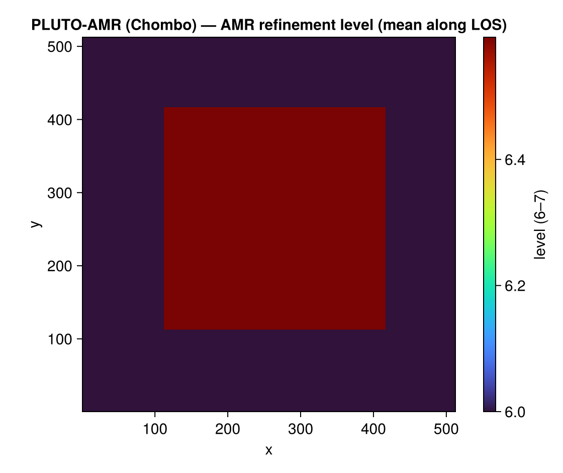

(HDF5 reading uses HDF5.jl, a dependency of Mera. Requires a power-of-two base grid and ref_ratio = 2, the common PLUTO/Chombo case.)

Reference readers

This frontend is built to agree with the origin tools — the readers that define PLUTO's formats:

• pyPLUTO — PLUTO's own Python reader, which documents the static-grid (grid.out + .dbl) layout. Mera's coordinate mapping is validated against it cell-for-cell.
• yt — reads PLUTO's Chombo-HDF5 AMR output through its chombo frontend, selecting sub-volumes lazily via data objects (ds.box, ds.sphere, ds.r[...]). Mera's load-time xrange/yrange/zrange mirrors that region-selector behaviour.

See also

• Multi-code support — the code-blind architecture and the sibling readers.
• getvar, projection, pdf, timeseries, getmovie — the analysis that runs on PLUTO data.