First Look

Two complementary ways to get a first impression of a simulation output:

• quicklook — a fixed, one-call dashboard (fast, budgeted): surface-density maps along each axis (plus stellar & dark-matter maps when particles are present), the ρ–T phase diagram, and a global census of cells, particles, masses and SFR.
• report — the composable form: you choose which cards (projections, phase diagrams, profiles, star-formation history, scalar totals/fractions, cross-datatype ratios) across any datatype, with a cost/runtime estimate beforehand and a wall-time budget.

Use quicklook for the instant overview; reach for report when you want to choose what goes in.

quicklook — the one-call dashboard

quicklook reads the header for instant facts and — unless you ask for header-only — does a single budgeted read to build the dashboard and print a compact summary:

using Mera
q = quicklook(80; path="/sim/cosmo")   # the cosmological zoom shown below

┌─ Mera quicklook ── output 80 (RAMSES) ───────────────
│ box        : 62140.0 kpc     levels 6–16  (finest 948.1 pc)
│ grid       : ndim 3 · ncpu 16 · nvarh 6
│ time       : -1574.0 Myr   z = 0.1426
│ particles  : 1090895 total  —  stars 31990 · DM 1058905
│ read       : 1058982 cells  ⚠ APPROXIMATE (coarse levels ≤ 9 of 16)
│ gas mass   : 2.21e15 M⊙  (approx.)
│ star mass  : 1.22e11 M⊙        DM mass : 1.134e16 M⊙
│ current SFR: 7.254 (10 Myr) · 4.381 (100 Myr) M⊙/yr
│ nH range   : 4.221e-9 … 5.798e-4 cm⁻³
│ T  range   : 45.13 … 3.933e7 K
│ figures    : .maps (Σ x,y,z + stars,dm)  ·  .phase (ρ–T)  ·  .budget (mass + SFR)
└─ 17.4 s ──────────────────────────────────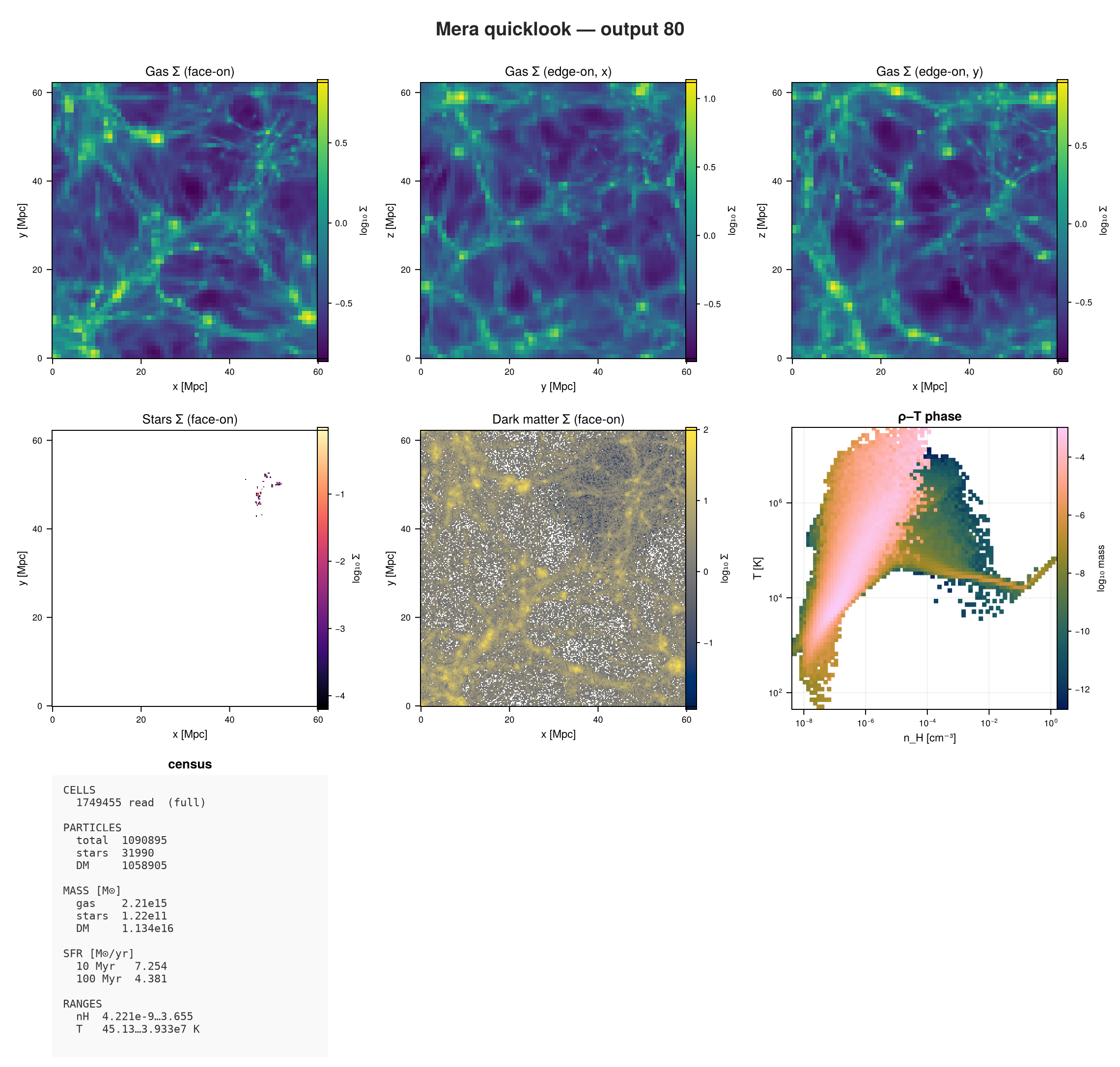

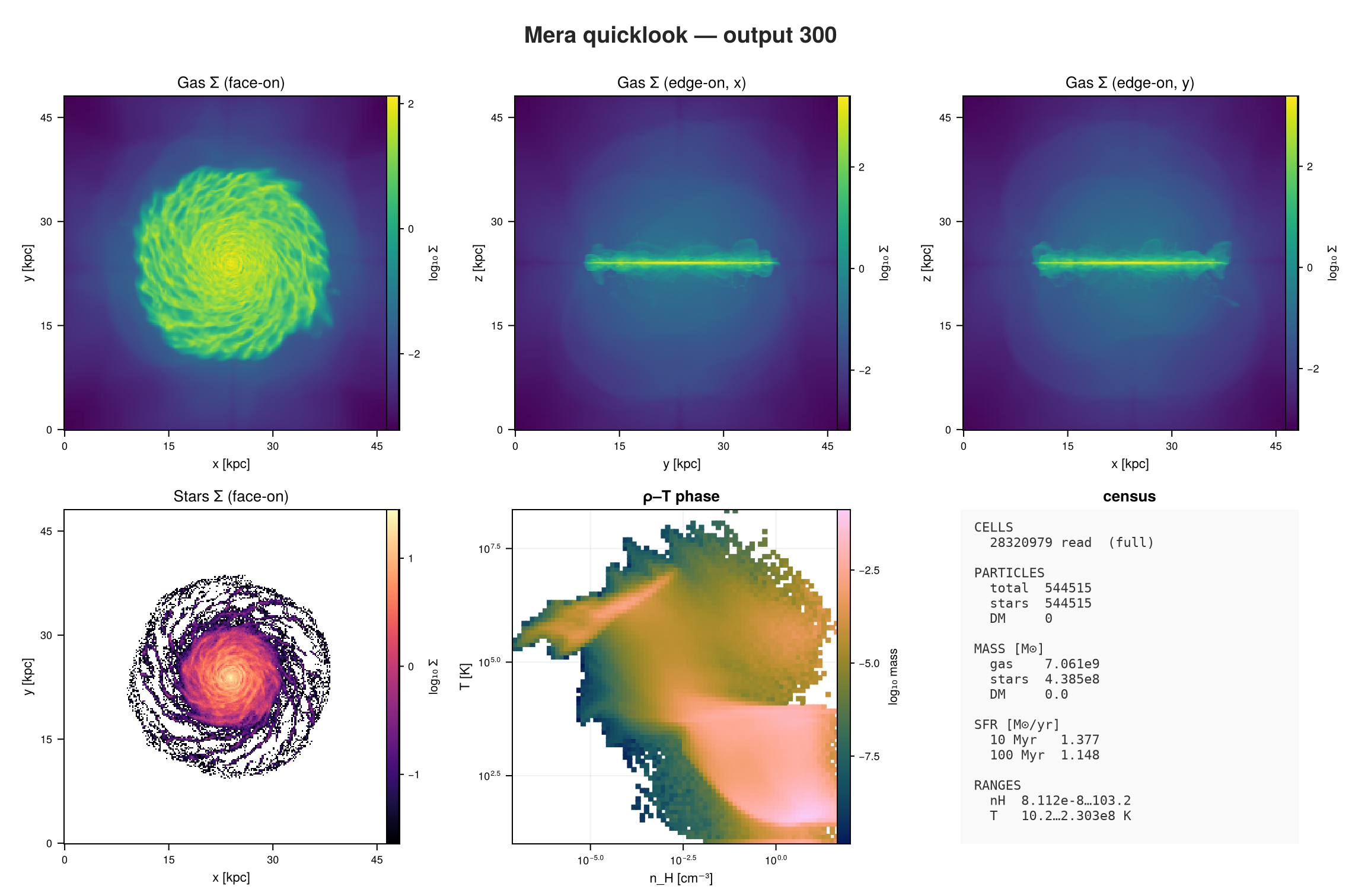
The same call on an isolated disk galaxy (gas + stars, no dark matter) — face-on plus the two edge-on views show the disk and its thickness, and the dark-matter panel is simply omitted:

What you get

The call returns a QuickLookResult:

• q.summary — header facts and estimates (box, levels, finest cell, time/redshift, the cell & particle census, masses, density/temperature ranges, read time).
• q.maps — surface-density projections: gas along each axis (q.maps.z/.x/.y, each an AMRMapsType with .maps[:sd]), plus face-on q.maps.stars / q.maps.dm when particles are present.
• q.phase — the ρ–T phase histogram (q.phase.H, q.phase.xedges, q.phase.yedges).
• q.budget — the global snapshot budget: gas_mass_Msol, and (with particles) stellar_mass_Msol, dm_mass_Msol, n_stars, n_dm, and the current SFR (sfr10, sfr100, sfr_mean, see sfr_snapshot).

Selecting components & projections

By default the dashboard shows every component present, with the three gas projections. Two keywords trim it to exactly what you want (and skip the reads you don't need):

• datatypes — any subset of [:hydro, :stars, :dm]. [:hydro] shows gas only; [:stars] or [:dm] show that population's face-on Σ and skip the gas read entirely (faster). The census and panels adapt to whatever was read.
• directions — any subset of [:z, :x, :y] for the gas maps (:z = face-on, :x/:y = edge-on). directions=[:z] gives a single face-on map — the most compact dashboard.

quicklook(300; path="/sim", directions=[:z])                 # one gas projection (compact)
quicklook(300; path="/sim", datatypes=[:hydro])              # gas only — no particle maps
quicklook(300; path="/sim", datatypes=[:stars])              # stellar map only (gas read skipped)
quicklook(300; path="/sim", datatypes=[:dm])                 # dark-matter map only
quicklook(300; path="/sim", datatypes=[:hydro, :stars], directions=[:z, :x])  # face-on + one edge-on

Budgeted reading — fast on big outputs

quicklook reads gas and particles differently, so it stays quick on large simulations:

• read=false — header only (sub-second): box, levels, finest cell, ncpu, fields, time/redshift, the particle census — no field data read.
• budget — a gas cell-count cap (default 2_000_000). If the full output is predicted larger, only the coarse AMR levels are read (spatially complete, lower resolution); the result is flagged sampled=true and gas-derived numbers are labelled approximate. lmax overrides the choice.
• Particles are read in full by default (a particle file is tiny next to the AMR hydro), which makes the stellar/DM mass and SFR exact even when the gas read is coarse.

quicklook(300; path="/sim/mw", read=false)        # instant header facts only
quicklook(300; path="/sim/mw", budget=500_000)    # cap the gas read on a huge output

Very large particle runs — particle_subsample

For runs where even reading all particle positions is the cost, particle_subsample reads only ~that fraction of the particle CPU files — skipping whole files, so it cuts both I/O and peak memory. RAMSES load-balances its domains to ~equal particles per CPU, so this reads ~that fraction of the particles; the census, masses and SFR are then scaled up by 1/fraction and flagged ⚠ approximate (an unbiased estimate for the total, noisier for rarer/clustered sub-populations):

quicklook(300; path="/sim/cosmo", particle_subsample=0.1)   # read ~10% of particle files

The same subsample keyword is available directly on getparticles (subsample=0.1); scale extensive quantities by 1/subsample for whole-snapshot estimates. For a localized region instead, getparticles(info; xrange=…) reads only the overlapping CPU domains.

Plotting

quicklookplot renders the multi-panel dashboard — gas Σ along x/y/z, face-on stellar & dark-matter Σ (when present), the ρ–T phase diagram, and a text census — with colorblind-safe colormaps (needs a Makie backend):

using CairoMakie
q   = quicklook(300; path="/sim/mw")
fig = quicklookplot(q)
CairoMakie.save("quicklook.png", fig)

report — composable cards

report turns a simulation output into one composable first-look summary: you pick which quantities and Mera functions to combine — projections, phase diagrams, profiles, star-formation history, scalar totals or fractions, cross-datatype ratios — across any datatype (hydro, particles, gravity, RT, clumps), and render the result as a text dashboard, a plot grid, or a saved file. Before it runs you get a cost/runtime estimate, and an optional budget keeps it within a wall-time target.

report(400; path="/sim")          # default: Σ map + ρ–T phase + disk ρ(R) profile + SFR history (ascii)

The no-argument default is the quicklook figures (gas Σ map · ρ–T phase · cylindrical density profile) plus a star-formation-history card — matching the star formation quicklook headlines in its census; the SFR card skips gracefully on an output without star particles. To compose your own, list cards:

report(400; path="/sim", output=:ascii, cards=[
    ProjectionCard(:hydro, :sd; unit=:Msol_pc2, res=512),                 # surface-density map
    PhaseCard(:hydro, :rho, :T; weight=:mass, xunit=:nH, yunit=:K),       # ρ–T phase diagram
    ProfileCard(:hydro, :r_cylinder, :rho; weight=:mass, nbins=40,        # disk radial density profile
                geometry=:cylindrical, center=[:bc], range_unit=:kpc, xunit=:kpc, unit=:nH, yscale=:log),
    ScalarCard(:hydro, :mass; reduce=:sum, unit=:Msol),                   # absolute gas mass
    ScalarCard(:hydro, :mass; fraction=true, label="cold_frac",           # cold-gas mass fraction
               mask = o -> getvar(o, :T, :K) .< 1e4),
    SFRCard(:particles; tbinsize=50.0),                                   # star-formation history
])

report reads each datatype once (with only the variables the cards actually need, via getvar_requirements), computes every card, and returns a QuickReport — which you can re-render or analyse further. With a Makie backend loaded, render(rep, :plot) lays the cards out as a figure grid:

using CairoMakie
rep = report(300; path="/sim", output=:none, cards=[ … ])
fig = render(rep, :plot; ncols=2)
CairoMakie.save("report.png", fig)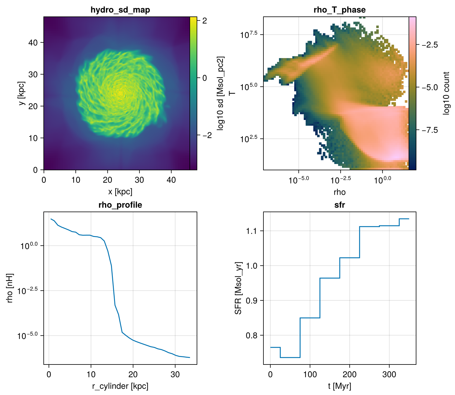

The cards

Each card names a datatype (first argument), a quantity, optional unit, and card-specific options. Any name getvar understands works — including your own add_field fields.

Absolute values vs fractions

Every aggregating card supports a fraction toggle. ScalarCard(...; fraction=true) divides by the total of relative_to (or the same variable); mask restricts the rows:

ScalarCard(:hydro, :mass; reduce=:sum, unit=:Msol)                        # absolute  [M⊙]
ScalarCard(:hydro, :mass; fraction=true, mask = o -> getvar(o,:T,:K).<1e4) # fraction of total

Profiles: geometry & axis scale

A ProfileCard's geometry sets the radial coordinate. For a disk galaxy use xvar=:r_cylinder, geometry=:cylindrical — radius in the disk plane — which is the default in the quicklook trio; a halo/spheroid is better with :r_sphere, geometry=:spherical. yscale controls the plotted y-axis: :log (log₁₀), :identity (linear), or :auto (log when the profile is positive and spans ≳ 1.5 decades, e.g. density). So the default density profile is cylindrical with a log y-axis.

ProfileCard(:hydro, :r_cylinder, :rho; geometry=:cylindrical, weight=:mass, unit=:nH, yscale=:log)  # disk
ProfileCard(:hydro, :r_sphere,   :rho; geometry=:spherical,   weight=:mass, unit=:nH)                # halo
ProfileCard(:hydro, :r_cylinder, :vz;  geometry=:cylindrical, weight=:mass, yscale=:identity)        # signed → linear

Star formation

SFRCard (and the standalone sfr) build the star-formation history from the star particles (birth ≠ 0): mode=:none gives M⊙/yr, mode=:probability the normalised SFH. For a single-number current SFR from one snapshot use sfr_snapshot — the stellar mass formed within a recent window divided by that window (e.g. 5/10/100 Myr), plus the lifetime mean. Both prefer a stored initial-mass field when present (mass=:auto), since the current particle mass underestimates the formed mass after stellar mass loss. Outputs without stars yield zeros, not an error.

Cross-datatype cards

CombinedCard reads several datatypes and combines them. Two are built in:

baryon_fraction()        # (gas + stars) / (gas + stars + dark matter)   [hydro + particles]
clump_mass_fraction()    # total clump mass / total gas mass             [clumps + hydro]

# your own:
CombinedCard([:hydro, :particles]; label="gas_to_star") do d
    sum(getvar(d[:hydro], :mass, :Msol)) / sum(getvar(d[:particles], :mass, :Msol))
end

Off-axis maps & custom fields

Projection cards take the same view controls as projection — direction=:faceon/:edgeon tilt the map to the disk (the report automatically reads the velocities needed to orient it):

ProjectionCard(:hydro, :sd; unit=:Msol_pc2, res=512, direction=:edgeon)   # edge-on Σ map

See Off-axis Projection for the full set of view options. Any field you register with add_field (see Derived Fields & add_field) is usable as a card quantity, and the report reads only its dependencies:

add_field(:vmag, (o,d) -> sqrt.(d[:vx].^2 .+ d[:vy].^2 .+ d[:vz].^2);
          depends_on=[:vx,:vy,:vz], unit=:km_s)
ProfileCard(:hydro, :r_cylinder, :vmag; weight=:mass, nbins=40)            # uses the custom field

Datatypes & graceful skipping

Scalar and profile cards work on hydro, particles, gravity, and clumps; projection cards work on hydro and particles (gravity/RT projection needs hydro pairing). A card is skipped with a note — never an error — when its datatype is absent from the output, or when it needs a variable that isn't stored (e.g. an RT :xHII card on a non-RT run). So a "kitchen-sink" plan runs unchanged on a hydro-only output.

report(output; path="/sim", cards=[ProjectionCard(:rt, :Np1; res=512)])   # photon density, group 1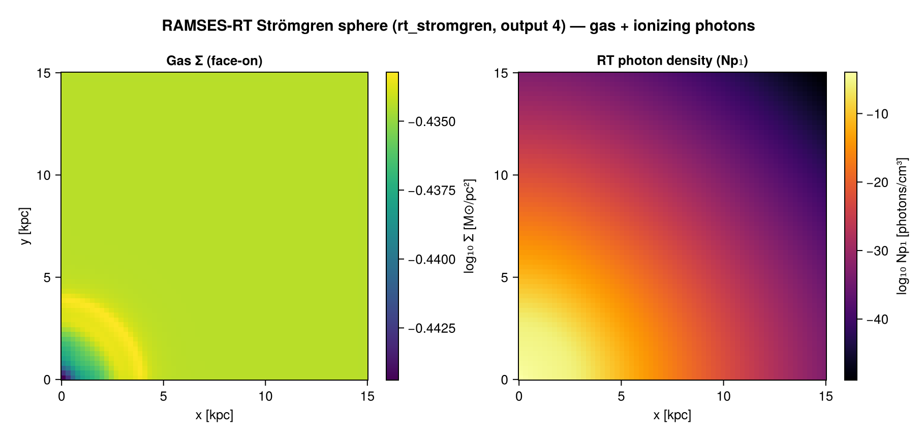

Cost estimate & budget

Inspect a plan's predicted cost with zero I/O before running:

plan = ReportPlan(400; path="/sim", cards=[...])
preview(plan)        # prints a per-card cells/time table + total
estimate(plan)       # the same numbers as a NamedTuple

The model self-calibrates — every real report learns this machine's timing; calibrate!(400; path="/sim") runs a quick active calibration. Keep a run within a wall-time target with the budget, which drops the read level first, then shrinks resolution/bins:

report(plan; budget_s=10.0)        # auto-fit ~10 s
downsample(plan, 10.0)             # or get the trimmed plan explicitly

Output backends

rep = report(plan; output=:none)          # compute only, render later
render(rep, :ascii)                        # text dashboard (default)
render(rep, :plot; ncols=2)                # Makie Figure grid  (needs `using CairoMakie`)
render(rep, :jld2; filename="r.jld2")      # full round-trip
render(rep, :file; mode=:dir, prefix="r")  # report.jld2 + summary.txt + one PNG per card
loadreport("r.jld2")                        # reload a saved QuickReport

Plotting lives in a package extension — load any Makie backend (using CairoMakie) and :plot / :file mode=:dir activate. Without one, those backends print a clear "load CairoMakie" message; everything else (ascii / jld2 / :file mode=:bundle) works with no extra dependencies.

Working with the result

rep.cards               # Vector{ReportResultCard}: each has .label .kind .datatype .data .meta
rep.cards[1].data.z     # e.g. the raw projection matrix — re-analyzable / re-plottable
rep.cost.per_card       # (label, seconds) per card
rep.summary             # header facts (box, levels, time/redshift, sampled?)
rep.provenance          # mera/julia version, timestamp, the plan

API

report(plan::ReportPlan; output=:ascii, budget_s=nothing, verbose=true)
report(sim_output::Int; path=".", cards=:default, output=:ascii, lmax=-1, budget=2_000_000, budget_s=nothing, verbose=true)

report(1; path=sim, output=:ascii, cards=[
    ProjectionCard(:hydro, :sd; unit=:Msol_pc2, res=512),
    PhaseCard(:hydro, :rho, :T; weight=:mass, xunit=:nH, yunit=:K),
    ScalarCard(:hydro, :mass; reduce=:sum, unit=:Msol),
])

preview(plan::ReportPlan; io=stdout) -> ReportPlan

estimate(plan::ReportPlan) -> NamedTuple

downsample(plan::ReportPlan, target_s) -> ReportPlan

calibrate!(output; path=".", budget=200_000) -> CostModel

render(report::QuickReport, backend::Symbol; kwargs...)

loadreport(filename) -> QuickReport

sfr(p::PartDataType; tbinsize=10.0, trange=[0.0, missing], mass=:auto, mask=[false],
    mode=:none, closed=:left) -> (t_Myr, sfr)

t, s = sfr(parts; tbinsize=50.0)            # SFR [M⊙/yr] vs t [Myr]
t, s = sfr(parts; mass=:minit)              # force a specific initial-mass field
t, s = sfr(parts; eta_sn=0.2)               # reconstruct birth mass from current mass (20% SN loss)

ProjectionCard(kind, var; unit=:standard, weight=:mass, res=256, direction=:z, center=[:bc], range_unit=:standard, label="")

PhaseCard(kind, xvar, yvar; weight=:mass, nbins=(80,80), xscale=:log, yscale=:log, xunit=:standard, yunit=:standard, label="")

ProfileCard(kind, xvar, yvar=nothing; weight=:mass, nbins=40, geometry=:none, unit=:standard, xunit=:standard, range_unit=:standard, center=[:bc], yscale=:auto, label="")

ScalarCard(kind, var; reduce=:sum, unit=:standard, fraction=false, relative_to=nothing, mask=nothing, label="")

SFRCard(kind=:particles; tbinsize=10.0, trange=[0.0,missing], unit=:Msol_yr, mode=:none, mass=:auto, mask=nothing, label="")

CombinedCard(datatypes, compute; unit=:fraction, label="combined")
CombinedCard(datatypes; unit=:fraction, label="combined") do datas … end

baryon_fraction(; label="baryon_fraction")

clump_mass_fraction(; label="clump_mass_fraction")

See also

• Derived Fields & add_field — register custom quantities usable as cards.
• Off-axis Projection — :faceon/:edgeon and arbitrary lines of sight.
• Profiles & Phase Diagrams — the profile/phase tools behind the cards.
• Star-Formation Rate — the standalone sfr / sfr_snapshot and the cosmological handling.