Time Series (multi-snapshot analysis)

Most post-processing is not about one snapshot — it is about evolution: how a mass, a peak density, a star-formation rate, or a profile changes across the outputs of a run. Writing that loop by hand (find the outputs, load each one, handle a missing snapshot, collect the numbers, keep memory under control) is boilerplate everyone re-implements.

timeseries turns it into a single call: you give it a reducer — a function that maps one loaded snapshot to a scalar or a NamedTuple — and it returns one tidy table with a row per output.

It works identically on raw RAMSES outputs and on mera (.jld2) files, and it loads one snapshot at a time — each is reduced and released before the next is read — so peak memory stays bounded on a laptop.

The idea, step by step

1. Discover the outputs in path (via checkoutputs for RAMSES, or a scan of output_*.jld2 for mera files). Select all of them, a range, or an explicit list.
2. Load output k — gethydro for RAMSES, loaddata for mera files. Only this one snapshot is in memory.
3. Reduce it: your reducer(d) returns the quantities you care about.
4. Append a row (output, time, …your fields…) to the result table; free the snapshot.
5. Analyse the resulting table — plot, fit, compare.

A real example: a 3-D Sedov blast

The fixture is a small Sedov point explosion (levelmin=5, levelmax=6, 13 outputs). One call gives the total mass, the peak density, and the AMR cell count at every output:

using Mera

ts = timeseries("/data/Mera-Tests/timeseries_sedov3d", d -> (
        mass    = msum(d, :Msol),
        rho_max = maximum(getvar(d, :rho)),
        ncells  = length(d.data),
     ); time_unit = :standard)        # this Sedov fixture is dimensionless → code-unit time

The result is an IndexedTables table — one row per output, with output and time columns added automatically (see Physical time — the default time is in Myr; the dimensionless Sedov sim is shown here in code units):

Table with 13 rows, 5 columns:
output  time       mass         rho_max  ncells
───────────────────────────────────────────────
1       0.0        6.28e-35     1.00     32768
2       0.0168     6.28e-35     2.46     81789
3       0.0335     6.28e-35     2.74     125371
⋮
12      0.1837     6.28e-35     7.27     261234
13      0.2004     6.28e-35     18.32    261969

Plotting those columns against time tells the whole story of the run at a glance:

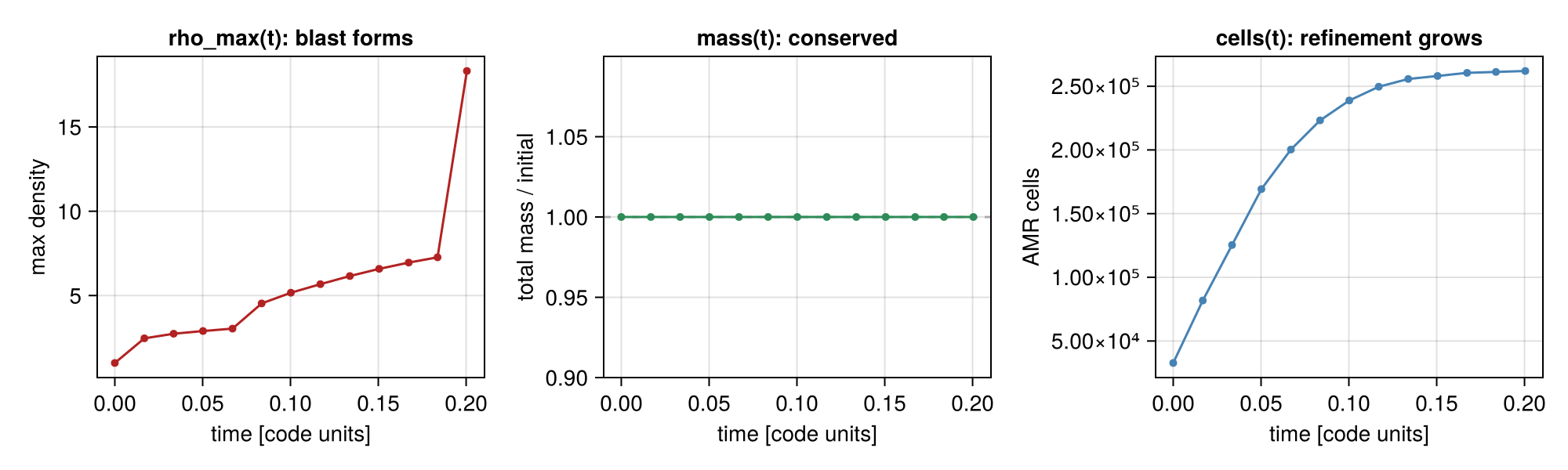
• rho_max(t) climbs as the shock steepens — the blast forms.
• mass(t) is flat: mass is conserved to round-off (the panel shows mass relative to its initial value, pinned at 1.0).
• ncells(t) grows from 32 768 to ~262 000 as the AMR mesh refines onto the expanding shock — a free diagnostic of how the grid is working.

Each column is a plain vector you can pull out with IndexedTables.columns:

using Mera.IndexedTables: columns
t   = columns(ts).time
rho = columns(ts).rho_max

Watching the blast evolve: projections over time

The reducer can return anything, so it can return a projection. This makes a projection a natural per-snapshot reduction: the small 2-D map is kept while the heavy AMR data of that snapshot is freed before the next is read. Reducing each output to its column-density map gives a time-series of maps — the frames of a movie:

movie = timeseries("/data/Mera-Tests/timeseries_sedov3d",
                   d -> projection(d, :sd, verbose=false).maps[:sd];
                   outputs = [1, 7, 13])

frames = columns(movie).value     # a vector of 2-D maps, one per output

Laid side by side, the maps show the shell sweeping outward through the box:

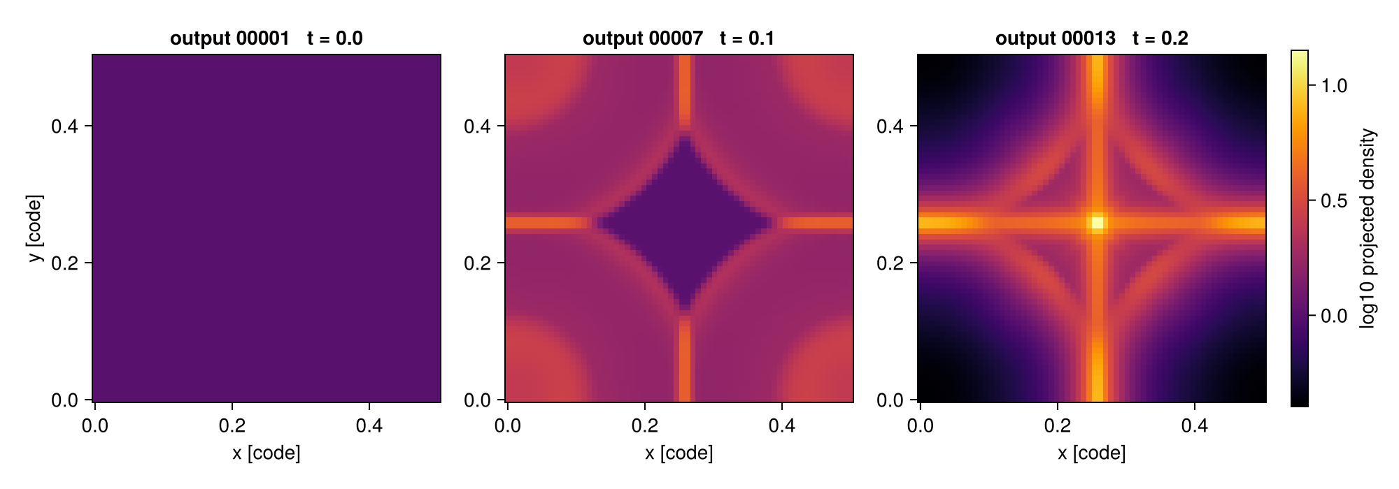
Return a scalar instead when you only need a number per snapshot — for example the peak column density over time, d -> maximum(projection(d, :sd, verbose=false).maps[:sd]).

Physical time and cosmological runs

The time column is physical by default — Myr (from gettime), not code units — so a time-series plots against a meaningful axis straight away. Choose another unit with time_unit (:Gyr, :yr, …), or time_unit = :standard for code units (as the dimensionless Sedov fixture above).

A cosmological run is detected automatically (iscosmological) and gets two extra columns — redshift (z = 1/aexp − 1) and aexp — so you can plot any quantity against redshift directly. The time column then holds the age of the universe in Myr:

ts = timeseries("/data/cosmo_run", d -> (sfr = …, mgas = msum(d, :Msol)))
# columns: output | time [Myr, = age] | redshift | aexp | sfr | mgas
using Mera.IndexedTables: columns
lines(columns(ts).redshift, columns(ts).mgas)     # gas mass vs redshift

Selecting which outputs

timeseries(path, reducer)                       # all outputs
timeseries(path, reducer; outputs = 1:5)        # a range
timeseries(path, reducer; outputs = [1,7,13])   # an explicit list

Numbers that are not present on disk are silently skipped, so a half-finished run or a gap in the output sequence is handled without special-casing.

Keeping memory bounded

timeseries already loads one snapshot at a time and frees it before the next. Two more levers cut the memory of each load — the main thing to reach for on a RAM-limited machine or with large outputs:

# read only up to AMR level 5, and only a sub-box around the centre
timeseries(path, d -> length(d.data);
           lmax = 5,
           xrange = [0.4, 0.6], yrange = [0.4, 0.6], zrange = [0.4, 0.6])

Snapshots are processed sequentially, so the loop never multiplies memory across outputs; the loaders themselves respect JULIA_NUM_THREADS (cap it at 4 on a laptop).

From mera files

If you have converted a run to mera files with savedata, point timeseries at the folder of output_*.jld2 files and set mera_files=true. The reducer and the resulting table are identical — mera files are typically several times smaller and faster to read:

timeseries("/data/Mera-Tests/timeseries_sedov3d_mera",
           d -> (mass = msum(d, :Msol), rho_max = maximum(getvar(d, :rho)));
           mera_files = true)

Masking and other Mera functions

The reducer receives the full data object for the snapshot, so anything that operates on a Mera data object composes inside it — there is nothing extra to wire up. That includes getvar, reductions like msum / center_of_mass / bulk_velocity, spatial selections like subregion / shellregion, projection (see above), and masking via the mask= keyword that most reductions accept.

For example, the mass of the dense gas (and its fraction) at every output — a boolean mask built from the snapshot and fed straight to msum:

ts = timeseries(path, d -> begin
        mask = getvar(d, :rho) .> 3.0                 # boolean mask over cells
        (m_total = msum(d, :Msol),
         m_dense = msum(d, :Msol, mask = mask),
         f_dense = msum(d, :Msol, mask = mask) / msum(d, :Msol))
     end)
# f_dense climbs 0.00 → 0.36 as the Sedov shock sweeps up and compresses gas

The same pattern covers "mass inside a sphere over time" (subregion(d, :sphere, …) then msum), "centre-of-mass drift" (center_of_mass), kinematics (bulk_velocity), and so on — each is just a one-line reducer.

Other data types — gravity, particles, clumps, RT

Set datatype to pick the loader. Radiative-transfer data (:rt) is a first-class type; mera files round-trip RT too (savedata/loaddata support it), so the mera path works the same way. On the Strömgren-sphere test run, the total photon density grows as the source ionizes its surroundings:

ts = timeseries("/data/Mera-Tests/rt_stromgren",
                d -> (np1 = sum(getvar(d, :Np1)),);   # group-1 photon density
                datatype = :rt)

For particles or clumps, use datatype=:particles / :clumps and reduce the relevant fields (e.g. d -> length(d.data) for a clump count, or a particle-mass sum).

A custom loader

For full control over how each snapshot is read — specific variables, a different data type, special keywords — pass a loader (info -> data). It overrides the built-in loading:

timeseries(path, d -> maximum(getvar(d, :rho));
           loader = info -> gethydro(info, [:rho]; lmax = 6))

Options

See also

• checkoutputs — list the outputs available in a run.
• gethydro, loaddata — the per-snapshot loaders.
• savedata — convert RAMSES outputs to mera files.
• gettime — the value in the time column.