Profiles & phase diagrams — a step-by-step guide
profile, phase, profile3d, rotationcurve and profiletimeseries are general, weighted reductions over any Mera field — a profile bins by one quantity (often a radius) and reports per-bin statistics of another; a phase diagram is a 2-D weighted histogram. They work on 3-D data (gas / gravity / particles) and on projected 2-D maps.
This guide builds the core features up one at a time, on one galaxy. Seven sections cover the essentials with a plot each; the remaining features share the same API and are summarised at the end.
Setup — load the galaxy once
Load hydro, gravity and clumps from one snapshot, plus a companion run that carries particles (dark matter + stars). Define a reusable physical center; profiles take a center in any length unit.
using Mera, CairoMakie
CairoMakie.activate!()
BASE = "/Volumes/FASTStorage/Simulations/Mera-Tests"   # <-- change me
info  = getinfo(100, joinpath(BASE,"spiral_clumps"), verbose=false)
gas   = gethydro(info,  verbose=false, show_progress=false)
grav  = getgravity(info, lmax=gas.lmax, verbose=false, show_progress=false)
parts = getparticles(getinfo(1, joinpath(BASE,"spiral_ugrid"), verbose=false), verbose=false, show_progress=false)
ctr = [:bc]                         # box centre; e.g. [24.,24.,24.] with range_unit=:kpc also works
println("gas cells = ", length(gas.data), "   particles = ", length(parts.data))
gas cells = 590311 particles = 454701. The simplest profile — binning a quantity
With only a bin field, profile returns the summed weight per bin — e.g. the radial mass profile M(R). The radius is measured about center; nbins, xrange, scale and units are physical. scale=:log gives log-spaced bins (the low edge is clamped to the smallest positive value; the top edge is inclusive). Set bins by count (nbins), by a physical width (binsize=0.5 in xunit, or binsize=(500,:pc) with its own unit; a dimensionless dex step under scale=:log), or by fully custom edges= — binsize/edges override nbins. Returns x (centres), edges, count, sum (Σweight), sumw2.
pl  = profile(gas, :r_cylinder; weight=:mass, nbins=50, xrange=(0,24), center=ctr, range_unit=:kpc, xunit=:kpc)
plg = profile(gas, :r_cylinder; weight=:mass, nbins=50, scale=:log, xrange=(0.3,24), center=ctr, range_unit=:kpc, xunit=:kpc)
pe  = profile(gas, :r_cylinder; weight=:mass, edges=[0.,2.,4.,8.,16.,24.], center=ctr, range_unit=:kpc, xunit=:kpc)
pbs = profile(gas, :r_cylinder; weight=:mass, binsize=(500,:pc), xrange=(0,24), center=ctr, range_unit=:kpc, xunit=:kpc)
println("binsize=(500,:pc) → bin width [kpc] = ", round(diff(pbs.edges)[1], digits=3), "  (", length(pbs.edges)-1, " bins)")
M(p) = p.sum .* gas.scale.Msol      # code mass -> Msol
fig = Figure(size=(1080,420))
ax1 = Axis(fig[1,1], xlabel="R [kpc]", ylabel="mass / bin [M⊙]", title="linear bins")
scatterlines!(ax1, pl.x, M(pl), color=:seagreen)
ax2 = Axis(fig[1,2], xscale=log10, yscale=log10, xlabel="R [kpc]", ylabel="mass / bin [M⊙]", title="log bins + custom edges")
o = M(plg) .> 0
lines!(ax2, plg.x[o], M(plg)[o], color=:dodgerblue, label="50 log bins")
stairs!(ax2, pe.x, max.(M(pe),1), color=:crimson, step=:center, label="custom edges")
axislegend(ax2, position=:rt); fig
binsize=(500,:pc) → bin width [kpc] = 0.5
(48 bins)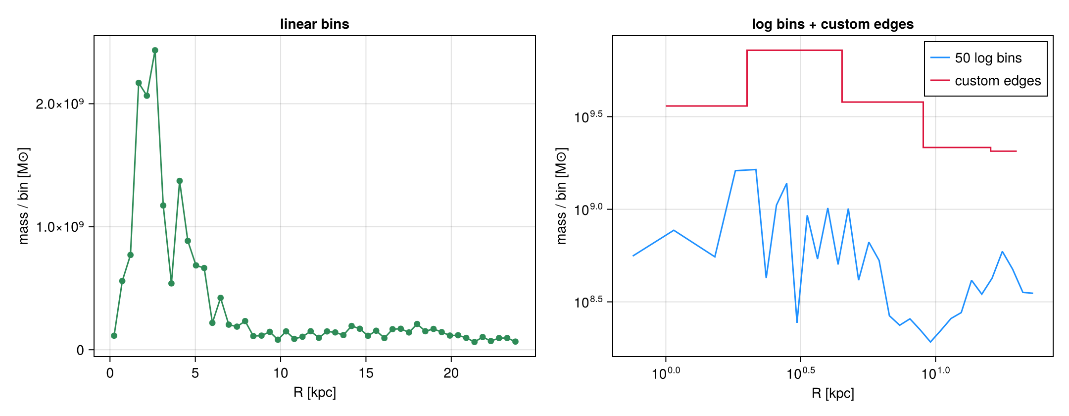
2. Per-bin statistics — a binned statistic is not a histogram
Give a second field yvar and each bin carries the weight-weighted mean, std, sem (standard error on the mean, std/√neff with the Kish effective sample size neff), min/max, median and a quantiles matrix at the requested qlevels. A custom statistic=f (called f(yview, wview) if it accepts weights, else f(yview)) adds a custom column. One figure makes the whole spread visible.
pT = profile(gas, :r_cylinder, :T; weight=:mass, unit=:K, nbins=35, xrange=(0,20), center=ctr, range_unit=:kpc, xunit=:kpc,
             quantiles=[0.16,0.5,0.84])
pC = profile(gas, :r_cylinder, :T; weight=:mass, unit=:K, nbins=35, xrange=(0,20), center=ctr, range_unit=:kpc, xunit=:kpc,
             statistic=(y,w)->sqrt(sum(w.*y.^2)/sum(w)))   # mass-weighted RMS -> pC.custom
ok = (pT.count .> 0) .& (pT.min .> 0) .& (pT.mean .> 0)
x=pT.x[ok]; mn=pT.min[ok]; mx=pT.max[ok]; q1=pT.quantiles[ok,1]; q3=pT.quantiles[ok,3]
mu=pT.mean[ok]; sd=pT.std[ok]; md_=pT.median[ok]; sem=pT.sem[ok]; rms=pC.custom[ok]; flo=minimum(mn)
fig = Figure(size=(760,500)); ax = Axis(fig[1,1], yscale=log10, xlabel="R [kpc]", ylabel="T [K]",
                                        title="temperature: mean, std, 16–84%, extrema, sem, custom RMS")
band!(ax, x, mn, mx, color=(:gray,0.15), label="min–max")
band!(ax, x, q1, q3, color=(:orange,0.30), label="16–84%")
band!(ax, x, max.(mu.-sd, flo), mu.+sd, color=(:dodgerblue,0.25), label="±std")
lines!(ax, x, md_, color=:black, linewidth=1.5, linestyle=:dash, label="median")
lines!(ax, x, mu, color=:dodgerblue, linewidth=2.5, label="mean")
lines!(ax, x, rms, color=:crimson, linewidth=2, label="custom RMS")
se = [i for i in 1:4:length(x) if mu[i]-sem[i] > 0]   # keep whiskers positive on the log axis
errorbars!(ax, x[se], mu[se], sem[se], color=:dodgerblue, whiskerwidth=6)
axislegend(ax, position=:rt, framevisible=false); fig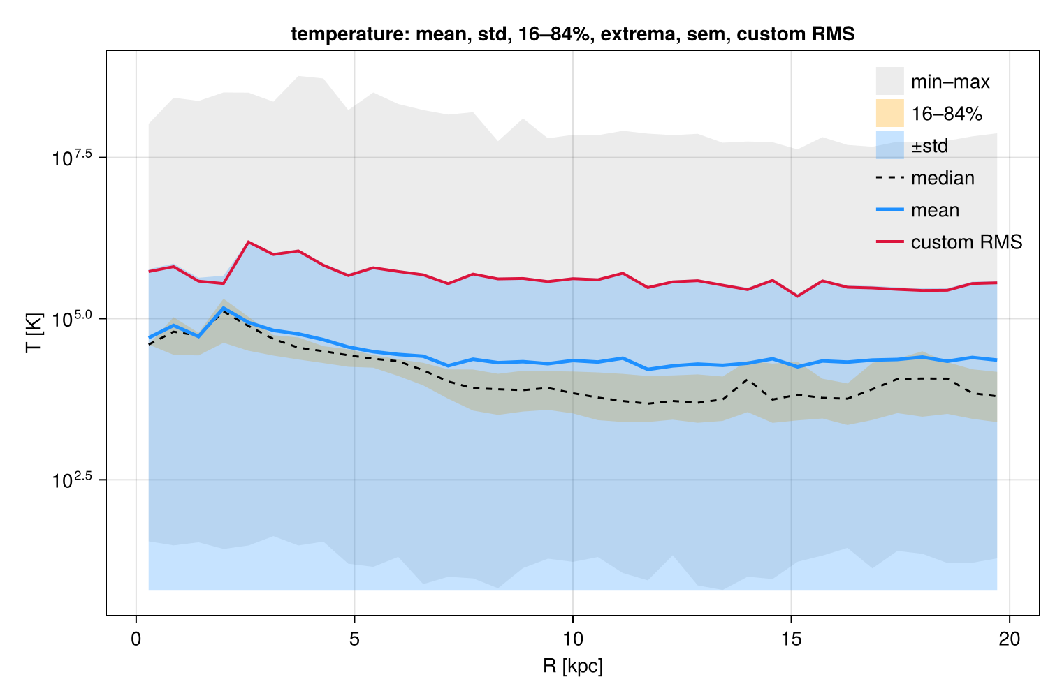
3. Density, enclosed mass & normalization (density PDF)
geometry=:spherical (shell 4/3·π·Δr³) or :cylindrical (annulus π·Δr²) divides the binned weight by the shell volume to give a physical density (weight-unit per xunit³, + shell_volume). cumulative=:forward (or :reverse) adds cumsum/cumcount — the enclosed mass M(<r). normalize=:sum gives per-bin fraction (Σ=1); normalize=:pdf gives a true probability density pdf (∫=1). The canonical use is the density PDF — bin by density and normalize; the weight then picks the mass-weighted vs volume-weighted ρ-PDF (they differ — the near-log-normal ISM density distribution).
pr = profile(gas, :r_sphere; weight=:mass, geometry=:spherical, cumulative=:forward, scale=:log,
             xrange=(0.3,24), nbins=40, center=ctr, range_unit=:kpc, xunit=:kpc)
ρ = pr.density .* gas.scale.Msol; Menc = pr.cumsum .* gas.scale.Msol
dm = profile(gas, :rho; weight=:mass,   normalize=:pdf, scale=:log, unit=:nH, nbins=60)   # mass-weighted ρ-PDF
dv = profile(gas, :rho; weight=:volume, normalize=:pdf, scale=:log, unit=:nH, nbins=60)   # volume-weighted ρ-PDF
fig = Figure(size=(1500,420))
ax1 = Axis(fig[1,1], xscale=log10, yscale=log10, xlabel="r [kpc]", ylabel="ρ [M⊙/kpc³]", title="spherical density ρ(r)  (geometry)")
od = ρ .> 0; scatterlines!(ax1, pr.x[od], ρ[od], color=:crimson)
ax2 = Axis(fig[1,2], xscale=log10, xlabel="r [kpc]", ylabel="M(<r) [M⊙]", title="enclosed mass  (cumulative)")
lines!(ax2, pr.x, Menc, color=:navy, linewidth=2.5)
ax3 = Axis(fig[1,3], xscale=log10, yscale=log10, xlabel="n_H [cm⁻³]", ylabel="pdf [per linear n_H]", title="density PDF  (normalize=:pdf)")
om = dm.pdf .> 0; ov = dv.pdf .> 0
lines!(ax3, dm.x[om], dm.pdf[om], color=:crimson, linewidth=2.5, label="mass-weighted")
lines!(ax3, dv.x[ov], dv.pdf[ov], color=:teal,    linewidth=2.5, label="volume-weighted")
axislegend(ax3, position=:lt); fig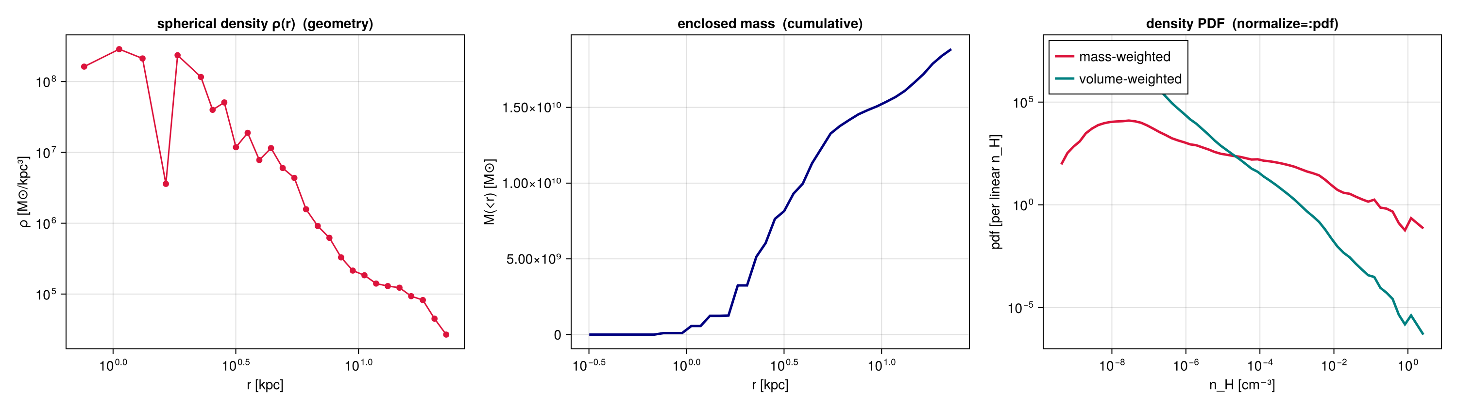
4. Weighting & components — mass vs volume vs none
weight is :mass, :volume (grid-only), :none (equal cells) or any field. Mass- and volume-weighted means differ wherever density varies within a bin; :none is the unweighted mean. Profiles work for every data type — but gravity/RT carry no :mass (use :volume/:none). To combine components, profile each on shared edges (here gas vs DM vs stars enclosed mass).
ed = collect(range(0,20,length=41))
pmw = profile(gas, :r_sphere, :rho; weight=:mass,   unit=:nH, edges=ed, center=ctr, range_unit=:kpc, xunit=:kpc)
pvw = profile(gas, :r_sphere, :rho; weight=:volume, unit=:nH, edges=ed, center=ctr, range_unit=:kpc, xunit=:kpc)
pep = profile(grav, :r_sphere, :epot; weight=:volume, edges=ed, center=ctr, range_unit=:kpc, xunit=:kpc)  # gravity: no :mass
fig = Figure(size=(1080,430))
ax1 = Axis(fig[1,1], yscale=log10, xlabel="r [kpc]", ylabel="⟨n_H⟩ [cm⁻³]", title="weighting: mass vs volume (gas)")
o1=(pmw.mean.>0); o2=(pvw.mean.>0)
lines!(ax1, pmw.x[o1], pmw.mean[o1], color=:crimson, linewidth=2.5, label="mass-weighted")
lines!(ax1, pvw.x[o2], pvw.mean[o2], color=:teal,    linewidth=2.5, label="volume-weighted")
axislegend(ax1, position=:rt)
ax2 = Axis(fig[1,2], xlabel="r [kpc]", ylabel="⟨Φ⟩ [code]", title="gravity potential (weight=:volume; no :mass)")
og=isfinite.(pep.mean); lines!(ax2, pep.x[og], pep.mean[og], color=:slateblue, linewidth=2.5); fig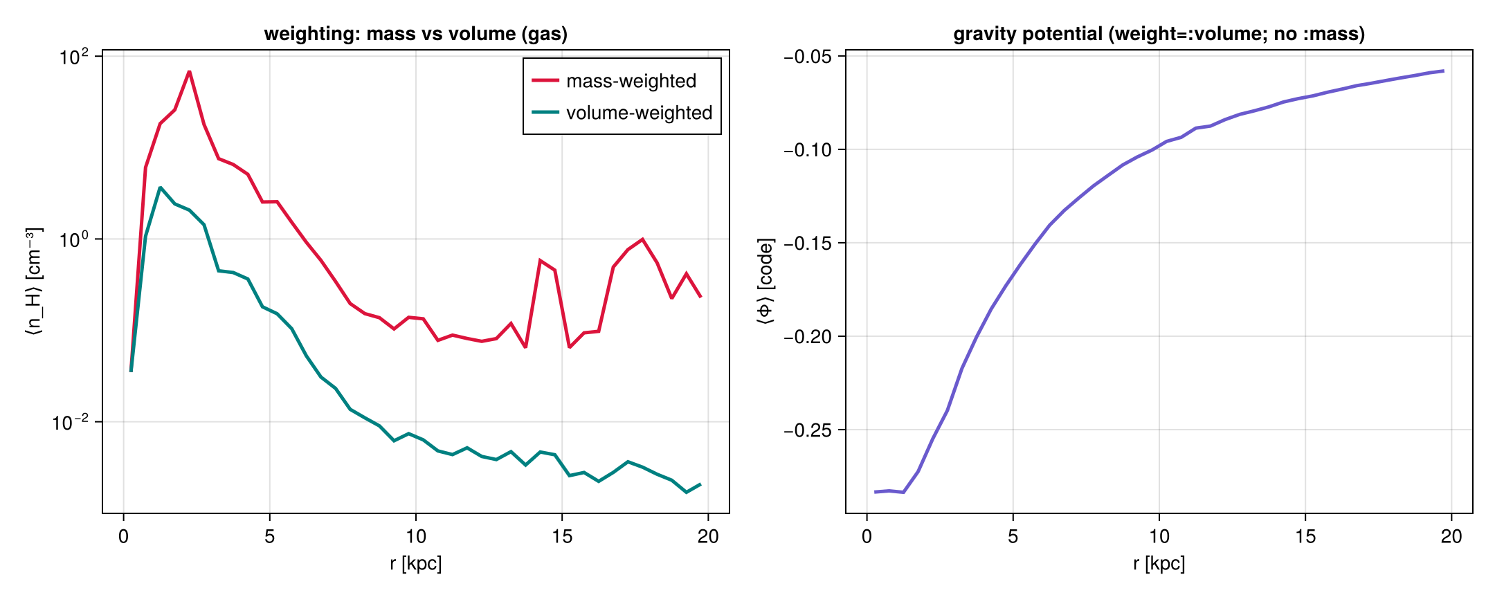
5. Rotation curve — who contributes how much
rotationcurve forms the enclosed mass M(<r) and returns the dynamical circular velocity v_circ = √(G·M(<r)/r). Run it per component — gas (optionally masked, e.g. cold gas only), stars, dark matter — and they add in quadrature, v_tot² = Σ v_i². The squared ratio (v_i/v_tot)² is exactly each component's fractional contribution to the rotational support. This is the dynamical mass decomposition (≠ the kinematic ⟨v_ϕ⟩ of §7).
How v_circ is estimated: the enclosed mass M(<r) is an exact direct sum of the binned masses; v_circ = √(G·M(<r)/r) is then the spherical (shell-theorem) idealization — it assumes spherical symmetry, so for a flattened disk it under-shoots at large R. The third panel overplots it against the exact curve from the solved gravity field, v = √(R·|a_R|) with a_R = getvar(grav, :ar_cylinder) (the true radial acceleration of all matter) — the dynamically rigorous rotation curve.
opts = (rvar=:r_cylinder, xunit=:kpc, center=ctr, range_unit=:kpc, nbins=50, xrange=(0.3,25))
rcg = rotationcurve(gas; opts...)                                  # all gas
cold = getvar(gas, :T, :K) .< 1e4                                  # a gas mask: cold gas (< 10⁴ K)
rcc = rotationcurve(gas; mask=cold, opts...)                       # cold-gas contribution
rcs = rotationcurve(parts; mask=getparticlemask(parts,:stars; verbose=false), opts...)
rcd = rotationcurve(parts; mask=getparticlemask(parts,:dm;    verbose=false), opts...)
vtot = sqrt.(rcg.v_circ.^2 .+ rcs.v_circ.^2 .+ rcd.v_circ.^2)       # spherical-estimate total
# EXACT curve from the solved gravity field: v = √(R·|a_R|), a_R = radial acceleration (all matter)
pa  = profile(grav, :r_cylinder, :ar_cylinder; weight=:volume, unit=:cm_s2, nbins=50, xrange=(0.3,25), center=ctr, range_unit=:kpc, xunit=:kpc)
Rcm = pa.x .* (Mera.getunit(info,:cm)/Mera.getunit(info,:kpc))
vexact = sqrt.(Rcm .* abs.(pa.mean)) ./ 1e5                        # km/s
fig = Figure(size=(1500,430))
ax1 = Axis(fig[1,1], xlabel="R [kpc]", ylabel="v_circ [km/s]", title="rotation curve by component")
lines!(ax1, rcd.x, rcd.v_circ, color=:navy,      linewidth=2, label="dark matter")
lines!(ax1, rcs.x, rcs.v_circ, color=:goldenrod, linewidth=2, label="stars")
lines!(ax1, rcg.x, rcg.v_circ, color=:seagreen,  linewidth=2, label="gas (all)")
lines!(ax1, rcc.x, rcc.v_circ, color=:seagreen,  linewidth=1.5, linestyle=:dot, label="gas (cold, masked)")
lines!(ax1, rcg.x, vtot, color=:black, linewidth=3, linestyle=:dash, label="total")
axislegend(ax1, position=:rb)
fd=(rcd.v_circ./vtot).^2; fs=(rcs.v_circ./vtot).^2; fg=(rcg.v_circ./vtot).^2
ax2 = Axis(fig[1,2], xlabel="R [kpc]", ylabel="(v_i / v_tot)²", title="fractional contribution to v²  (stacks to 1)")
band!(ax2, rcg.x, fill(0.0,length(rcg.x)), fd, color=(:navy,0.6), label="dark matter")
band!(ax2, rcg.x, fd, fd.+fs, color=(:goldenrod,0.6), label="stars")
band!(ax2, rcg.x, fd.+fs, fd.+fs.+fg, color=(:seagreen,0.6), label="gas")
axislegend(ax2, position=:rc)
ax3 = Axis(fig[1,3], xlabel="R [kpc]", ylabel="v_circ [km/s]", title="spherical estimate vs exact (from ∂Φ)")
lines!(ax3, rcg.x, vtot, color=:gray, linewidth=2.5, label="√(GM(<r)/r)  (spherical)")
lines!(ax3, pa.x, vexact, color=:crimson, linewidth=2.5, label="√(R·|a_R|)  (gravity, exact)")
axislegend(ax3, position=:rb); fig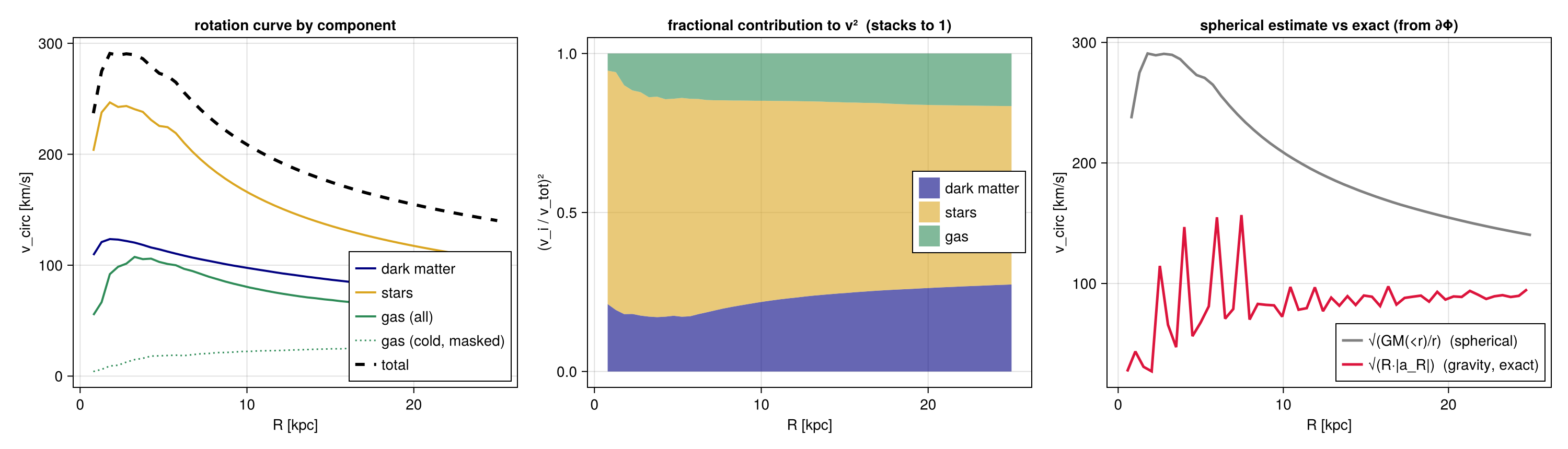
6. Phase diagrams — colour is a knob
phase is a 2-D weighted histogram of two fields — the classic mass-weighted ρ–T diagram. With a third field cvar each cell is coloured by the per-cell weighted mean; cstat swaps that for :std/:median/:min/:max/:full or a function. normalize=:pdf makes a 2-D PDF, and xedges/yedges accept custom edges. Same ρ–T plane, four different colourings:
kw = (weight=:mass, nbins=(140,140), xscale=:log, yscale=:log, xunit=:nH, yunit=:K, center=ctr, range_unit=:kpc)
ph  = phase(gas, :rho, :T; kw...)
pcv = phase(gas, :rho, :T, :vϕ_cylinder; cstat=:mean, cunit=:km_s, kw...)
psd = phase(gas, :rho, :T, :vϕ_cylinder; cstat=:std,  cunit=:km_s, kw...)   # also :median/:min/:max/:full/callable
ppdf= phase(gas, :rho, :T; normalize=:pdf, kw...)
xc = log10.((ph.xedges[1:end-1].+ph.xedges[2:end])./2)
yc = log10.((ph.yedges[1:end-1].+ph.yedges[2:end])./2)
lg(M)=log10.(replace(M,0.0=>NaN)); fig=Figure(size=(1150,860))
for (k,(lab,M,cm,fn)) in enumerate((("mass (H)",ph.H,:magma,lg),("⟨v_ϕ⟩ [km/s]",pcv.mean,:balance,identity),
                                    ("σ(v_ϕ) [km/s]",psd.std,:viridis,identity),("PDF",ppdf.pdf,:magma,lg)))
    r=(k-1)÷2+1; c=2*((k-1)%2)+1
    ax=Axis(fig[r,c], xlabel="log₁₀ n_H [cm⁻³]", ylabel="log₁₀ T [K]", title=lab)
    A=fn(M); hm=heatmap!(ax, xc, yc, A, colormap=cm, nan_color=:black); Colorbar(fig[r,c+1], hm)
end
fig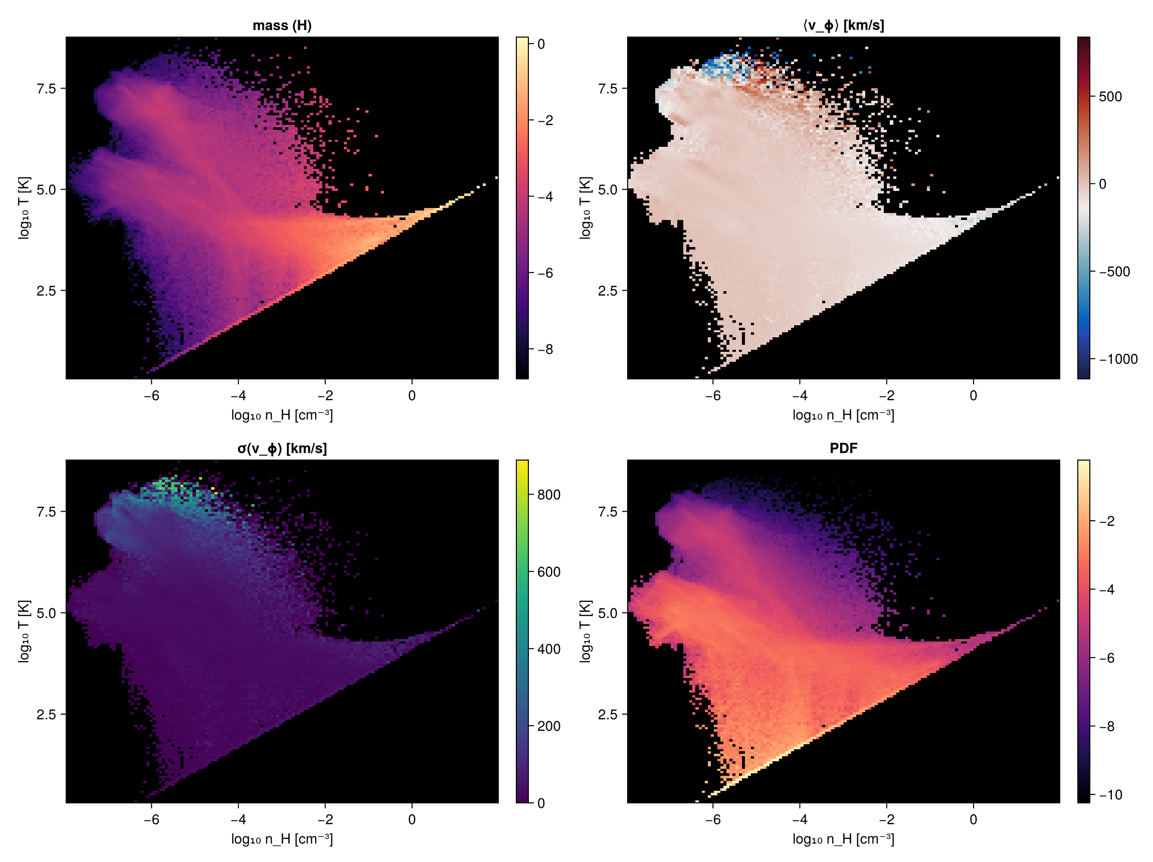
7. Distribution shape & uncertainties — moments, equal-count bins, bootstrap CIs
Three statistics upgrades, all opt-in and composable:
skewnessand (excess)kurtosisare always returned with ayvar— the asymmetry and tail-weight of each bin's distribution (a Gaussian gives both ≈ 0).scale=:equalplaces quantile-spaced edges so every bin holds about the same number of points — far steadier statistics where the disk thins out (vs fixed-width bins that empty out).bootstrap=Nresamples each bin to add confidence intervals for the per-bin mean and median (mean_ci/median_ci,nbins×2) plusmedian_se;ci=:percentile(default),:basicor:bca(bias-corrected & accelerated). It is deterministic (seeded), so reruns match.
pe = profile(gas, :r_cylinder, :vz; weight=:mass, unit=:km_s, scale=:equal, nbins=18,
             center=ctr, range_unit=:kpc, xunit=:kpc, bootstrap=800, ci=:bca, confidence_level=0.95)
println("equal-count points/bin (min..max): ", extrema(pe.count), "  → nearly equal")
ok = pe.count .> 5
x = pe.x[ok]; mu = pe.mean[ok]; lo = pe.mean_ci[ok,1]; hi = pe.mean_ci[ok,2]
sk = pe.skewness[ok]; ku = pe.kurtosis[ok]
fig = Figure(size=(900,420))
ax1 = Axis(fig[1,1], xlabel="R [kpc]", ylabel="⟨v_z⟩ [km/s]", title="equal-count bins + BCa bootstrap 95% CI")
band!(ax1, x, lo, hi, color=(:dodgerblue,0.25), label="95% CI (bootstrap)")
lines!(ax1, x, mu, color=:dodgerblue, linewidth=2.5, label="⟨v_z⟩")
axislegend(ax1, position=:rt, framevisible=false)
ax2 = Axis(fig[1,2], xlabel="R [kpc]", ylabel="shape moment", title="shape of the v_z distribution per bin")
hlines!(ax2, [0.0], color=:gray, linestyle=:dash)
lines!(ax2, x, sk, color=:crimson, linewidth=2, label="skewness")
lines!(ax2, x, ku, color=:seagreen, linewidth=2, label="excess kurtosis")
axislegend(ax2, position=:rt, framevisible=false); fig
equal-count points/bin (min..max): (
32300, 33260) → nearly equal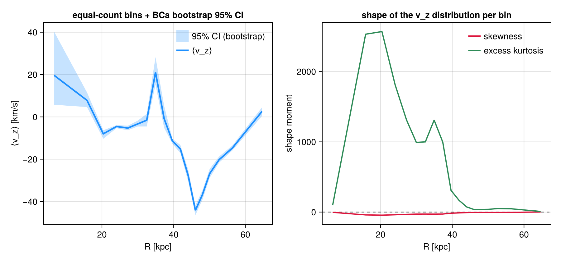
More features (same API, no separate plot here)
These use exactly the same profile/phase calls shown above:
- Many fields in one pass — pass
yvaras a vector to bin once and reduce several fields together (cheaper than one call per field); per-field stats live underp.fields[:T], inp.yvarsorder:profile(gas, :r_cylinder, [:T, :rho]; weight=:mass, nbins=40, center=ctr, range_unit=:kpc). - Velocity decomposition —
getvarsplits each cell's velocity aboutcenterinto:vr_cylinder(radial in/outflow, ±),:vϕ_cylinder(rotation),:vz(vertical), plus the spherical triplet:vr_sphere/:vθ_sphere/:vϕ_sphere. Profiling them gives ⟨v⟩(R) (mean, signed) and the rest-frame dispersion σ(R) (std, about the per-bin mean, so net rotation doesn't inflate it).velocitydispersionreturns σR/σϕ/σz and the total σ in one call. These are 3-D, per-annulus dispersions about the bin mean (intra-bin shear retained); for a local, per-pixel line-of-sight dispersion use the projected:σlosmap instead — `profile(projection(gas, :σlos, :kms; direction=:edgeon, center=ctr, range_unit=:kpc), :σlos; xvar=:r, weight=:sd)`. - Select particles —
getparticlemask(parts, :stars)(or:dm/:clouds/… , a familyInt, or(family=…, tag=…)) builds a boolean mask to pass asmask=to any profile call. - Profiles from a 2-D map —
profilealso takes aprojectionresult: bin map pixels by image-plane radius:r(a surface brightness Σ(R)), by:x/:y, or by another map; weight by:none/:areaor a map key. Works for off-axis (e.g. edge-on) maps too —:rstays centred on the object.profile(proj, :sd; xvar=:r, weight=:none, xunit=:kpc, nbins=30). - 3-D profiles —
profile3d(gas, :rho, :T, :z; weight=:mass, nbins=(80,80,24), …)bins by three fields; marginalizing one axis reproducesphaseexactly (a built-in consistency check). - Evolution across snapshots —
profiletimeseries(loadfn, outputs, xvar, yvar; …)stacks a profile over many outputs into an(nbins × n_snapshots)matrix on a fixed radius axis.
Takeaway
| feature | call |
|---|---|
bin a quantity; log/custom edges | profile(obj, x) |
| per-bin mean/std/sem/quantiles/min/max/custom | profile(obj, x, y; statistic=…) |
| density / enclosed mass / fraction / pdf | geometry, cumulative, normalize |
| many fields in one pass | profile(obj, x, [y1,y2]) → .fields |
| mass/volume/none/field weighting; components | weight=…, shared edges |
| rotation curve — gas (maskable) / stars / DM | rotationcurve(obj; mask=…) |
| velocity decomposition ⟨vϕ⟩/⟨vr⟩ + σr/σϕ/σ_z | profile(obj, r, :vϕ_cylinder/:vr_cylinder/:vz) |
| select particles by type/family/tag | getparticlemask |
| profile from a 2-D map (Σ(R), map-weighted) | profile(m::DataMapsType, …) |
| 2-D phase; colour by mean/std/…; PDF | phase(obj, x, y[, c]; cstat, normalize) |
| 3-D histogram; marginal == phase | profile3d |
| radius-vs-time evolution | profiletimeseries |
| distribution shape; equal-count bins; bootstrap CIs | skewness/kurtosis, scale=:equal, bootstrap=N |
Profiles & phase work on gas, gravity, particles and projected maps (source=:data or :map). Everything here is regression-tested in the Mera test suite. For line-of-sight distributions (per-pixel spectra, velocity cubes) see the Off-axis Projection guide.