3. Particles: Get Sub-Regions of Loaded the Data
Load the Data
using Mera, PyPlot
using ColorSchemes
cmap = ColorMap(ColorSchemes.lajolla.colors) # See http://www.fabiocrameri.ch/colourmaps.php

info = getinfo(400, "/Volumes/FASTStorage/Simulations/Mera-Tests/manu_sim_sf_L14");
particles = getparticles(info, :mass); [Mera]: 2025-06-30T20:24:04.066
Code: RAMSES
output [400] summary:
mtime: 2018-09-05T09:51:55
ctime: 2025-06-29T20:06:45.267
=======================================================
simulation time: 594.98 [Myr]
boxlen: 48.0 [kpc]
ncpu: 2048
ndim: 3
-------------------------------------------------------
amr: true
level(s): 6 - 14 --> cellsize(s): 750.0 [pc] - 2.93 [pc]
-------------------------------------------------------
hydro: true
hydro-variables: 7 --> (:rho, :vx, :vy, :vz, :p, :var6, :var7)
hydro-descriptor: (:density, :velocity_x, :velocity_y, :velocity_z, :thermal_pressure, :passive_scalar_1, :passive_scalar_2)
γ: 1.6667
-------------------------------------------------------
gravity: true
gravity-variables: (:epot, :ax, :ay, :az)
-------------------------------------------------------
particles: true
- Npart: 5.091500e+05
- Nstars: 5.066030e+05
- Ndm: 2.547000e+03
particle-variables: 5 --> (:vx, :vy, :vz, :mass, :birth)
-------------------------------------------------------
rt: false
-------------------------------------------------------
clumps: true
clump-variables: (:index, :lev, :parent, :ncell, :peak_x, :peak_y, :peak_z, Symbol("rho-"), Symbol("rho+"), :rho_av, :mass_cl, :relevance)
-------------------------------------------------------
namelist-file: false
timer-file: false
compilation-file: true
makefile: true
patchfile: true
=======================================================
[Mera]: Get particle data: 2025-06-30T20:24:04.247
Key vars=(:level, :x, :y, :z, :id)
Using var(s)=(4,) = (:mass,)
domain:
xmin::xmax: 0.0 :: 1.0 ==> 0.0 [kpc] :: 48.0 [kpc]
ymin::ymax: 0.0 :: 1.0 ==> 0.0 [kpc] :: 48.0 [kpc]
zmin::zmax: 0.0 :: 1.0 ==> 0.0 [kpc] :: 48.0 [kpc]
Progress: 100%|█████████████████████████████████████████| Time: 0:00:19
Found 5.089390e+05 particles
Memory used for data table :19.415205001831055 MB
-------------------------------------------------------Cuboid Region
Create projections of the full box:
proj_z = projection(particles, :sd, unit=:Msol_pc2, center=[:boxcenter], direction=:z, lmax=8, verbose=false);
proj_y = projection(particles, :sd, unit=:Msol_pc2, center=[:boxcenter], direction=:y, lmax=8, verbose=false);
proj_x = projection(particles, :sd, unit=:Msol_pc2, center=[:boxcenter], direction=:x, lmax=8, verbose=false);
The generated objects include, e.g. the extent of the processed domain, that can be used to declare the specific range of the plots, while the field cextent gives the extent related to a given center (default: [0.,0.,0.]).
propertynames(proj_z)(:maps, :maps_unit, :maps_lmax, :maps_mode, :lmax_projected, :lmin, :lmax, :ref_time, :ranges, :extent, :cextent, :ratio, :effres, :pixsize, :boxlen, :scale, :info)Cuboid Region: The red lines show the region that we want to cutout as a sub-region from the full data:
figure(figsize=(15.5, 3.5))
labeltext = L"\mathrm{log10(\Sigma) \ [M_{\odot} pc^{-2}]}"

subplot(1,3,1)
im = imshow( log10.( permutedims(proj_z.maps[:sd]) ), cmap=cmap, aspect=proj_z.ratio, origin="lower", extent=proj_z.cextent, vmin=0, vmax=3)
plot([-4.,0.,0.,-4.,-4.],[-15.,-15.,15.,15.,-15.], color="red")
xlabel("x [kpc]")
ylabel("y [kpc]")
cb = colorbar(im, label=labeltext)

subplot(1,3,2)
im = imshow( log10.( permutedims(proj_y.maps[:sd]) ), cmap=cmap, aspect=proj_y.ratio, origin="lower", extent=proj_y.cextent, vmin=0, vmax=3)
plot([-4.,0.,0.,-4.,-4.],[-2.,-2.,2.,2.,-2.], color="red")
xlabel("x [kpc]")
ylabel("z [kpc]")
cb = colorbar(im, label=labeltext)

subplot(1,3,3)
im = imshow( log10.( permutedims(proj_x.maps[:sd]) ), cmap=cmap, aspect=proj_x.ratio, origin="lower", extent=proj_x.cextent, vmin=0, vmax=3)
plot([-15.,15.,15.,-15.,-15.],[-2.,-2.,2.,2.,-2.], color="red")
xlabel("y [kpc]")
ylabel("z [kpc]")
cb = colorbar(im, label=labeltext);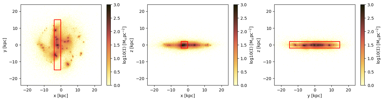
Cuboid Region: Cutout the data assigned to the object particles
Note: The selected regions can be given relative to a user given center or to the box corner [0., 0., 0.] by default. The user can choose between standard notation [0:1] (default) or physical length-units, defined in e.g. info.scale :
part_subregion = subregion( particles, :cuboid,
                                    xrange=[-4., 0.],
                                    yrange=[-15. ,15.],
                                    zrange=[-2. ,2.],
                                    center=[:boxcenter],
range_unit=:kpc );[Mera]: 2025-06-30T20:24:24.755
center: [0.5, 0.5, 0.5] ==> [24.0 [kpc] :: 24.0 [kpc] :: 24.0 [kpc]]
domain:
xmin::xmax: 0.4166667 :: 0.5 ==> 20.0 [kpc] :: 24.0 [kpc]
ymin::ymax: 0.1875 :: 0.8125 ==> 9.0 [kpc] :: 39.0 [kpc]
zmin::zmax: 0.4583333 :: 0.5416667 ==> 22.0 [kpc] :: 26.0 [kpc]
Memory used for data table :10.259893417358398 MB
-------------------------------------------------------The function subregion creates a new object with the same type as the object created by the function getparticles :
typeof(part_subregion)PartDataTypeCuboid Region: Projections of the sub-region.
The coordinates center is the center of the box:
proj_z = projection(part_subregion, :sd, unit=:Msol_pc2, center=[:boxcenter], direction=:z, lmax=10, verbose=false);
proj_y = projection(part_subregion, :sd, unit=:Msol_pc2, center=[:boxcenter], direction=:y, lmax=10, verbose=false);
proj_x = projection(part_subregion, :sd, unit=:Msol_pc2, center=[:boxcenter], direction=:x, lmax=10, verbose=false);
figure(figsize=(15.5, 3.5))
labeltext = L"\mathrm{log10(\Sigma) \ [M_{\odot} pc^{-2}]}"
subplot(1,3,1)
im = imshow( log10.( permutedims(proj_z.maps[:sd]) ), cmap=cmap, origin="lower", extent=proj_z.cextent, vmin=0, vmax=3)
xlabel("x [kpc]")
ylabel("y [kpc]")
cb = colorbar(im, label=labeltext)
subplot(1,3,2)
im = imshow( log10.( permutedims(proj_y.maps[:sd]) ), cmap=cmap, origin="lower", extent=proj_y.cextent, vmin=0, vmax=3)
xlabel("x [kpc]")
ylabel("z [kpc]")
cb = colorbar(im, label=labeltext)
subplot(1,3,3)
im = imshow( log10.( permutedims(proj_x.maps[:sd]) ), cmap=cmap, origin="lower", extent=proj_x.cextent, vmin=0, vmax=3)
xlabel("y [kpc]")
ylabel("z [kpc]")
cb = colorbar(im, orientation="horizontal", label=labeltext, pad=0.2);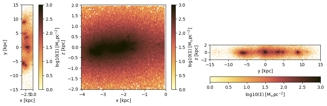
Cuboid Region: Get the data outside of the selected region (inverse selection):
part_subregion = subregion( particles, :cuboid,
                                    xrange=[-4., 0.],
                                    yrange=[-15. ,15.],
                                    zrange=[-2. ,2.],
                                    center=[24.,24.,24.],
                                    range_unit=:kpc,
inverse=true);[Mera]: 2025-06-30T20:24:25.248
center: [0.5, 0.5, 0.5] ==> [24.0 [kpc] :: 24.0 [kpc] :: 24.0 [kpc]]
domain:
xmin::xmax: 0.4166667 :: 0.5 ==> 20.0 [kpc] :: 24.0 [kpc]
ymin::ymax: 0.1875 :: 0.8125 ==> 9.0 [kpc] :: 39.0 [kpc]
zmin::zmax: 0.4583333 :: 0.5416667 ==> 22.0 [kpc] :: 26.0 [kpc]
Memory used for data table :9.156034469604492 MB
-------------------------------------------------------proj_z = projection(part_subregion, :sd, unit=:Msol_pc2, center=[:boxcenter], direction=:z, lmax=8, verbose=false);
proj_y = projection(part_subregion, :sd, unit=:Msol_pc2, center=[:boxcenter], direction=:y, lmax=8, verbose=false);
proj_x = projection(part_subregion, :sd, unit=:Msol_pc2, center=[:boxcenter], direction=:x, lmax=8, verbose=false);figure(figsize=(15.5, 3.5))
labeltext = L"\mathrm{log10(\Sigma) \ [M_{\odot} pc^{-2}]}"
subplot(1,3,1)
im = imshow( log10.( permutedims(proj_z.maps[:sd]) ), cmap=cmap, aspect=proj_z.ratio, origin="lower", extent=proj_z.cextent, vmin=0, vmax=3)
plot([-4.,0.,0.,-4.,-4.],[-15.,-15.,15.,15.,-15.], color="red")
xlabel("x [kpc]")
ylabel("y [kpc]")
cb = colorbar(im, label=labeltext)
subplot(1,3,2)
im = imshow( log10.( permutedims(proj_y.maps[:sd]) ), cmap=cmap, aspect=proj_y.ratio, origin="lower", extent=proj_y.cextent, vmin=0, vmax=3)
plot([-4.,0.,0.,-4.,-4.],[-2.,-2.,2.,2.,-2.], color="red")
xlabel("x [kpc]")
ylabel("z [kpc]")
cb = colorbar(im, label=labeltext)
subplot(1,3,3)
im = imshow( log10.( permutedims(proj_x.maps[:sd]) ), cmap=cmap, aspect=proj_x.ratio, origin="lower", extent=proj_x.cextent, vmin=0, vmax=3)
plot([-15.,15.,15.,-15.,-15.],[-2.,-2.,2.,2.,-2.], color="red")
xlabel("y [kpc]")
ylabel("z [kpc]")
cb = colorbar(im, label=labeltext);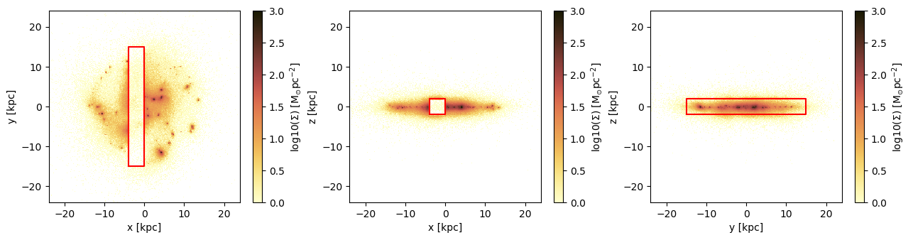
Cylindrical Region
Create projections of the full box:
proj_z = projection(particles, :sd, unit=:Msol_pc2, center=[:boxcenter], direction=:z, lmax=8, verbose=false);
proj_y = projection(particles, :sd, unit=:Msol_pc2, center=[:boxcenter], direction=:y, lmax=8, verbose=false);
proj_x = projection(particles, :sd, unit=:Msol_pc2, center=[:boxcenter], direction=:x, lmax=8, verbose=false);Cylindrical Region: The red lines show the region that we want to cutout as a sub-region from the full data:
figure(figsize=(15.5, 3.5))
labeltext = L"\mathrm{log10(\Sigma) \ [M_{\odot} pc^{-2}]}"
theta = range(-pi, stop=pi, length=100)
subplot(1,3,1)
im = imshow( log10.( permutedims(proj_z.maps[:sd]) ), cmap=cmap, aspect=proj_z.ratio, origin="lower", extent=proj_z.cextent, vmin=0, vmax=3)
plot( 3. .* sin.(theta) .-11, 3 .* cos.(theta), color="red")
xlabel("x [kpc]")
ylabel("y [kpc]")
cb = colorbar(im, label=labeltext)
subplot(1,3,2)
im = imshow( log10.( permutedims(proj_y.maps[:sd]) ), cmap=cmap, origin="lower", extent=proj_y.cextent, vmin=0, vmax=3)
plot([-3.,3.,3.,-3.,-3.] .-11.,[-2.,-2.,2.,2.,-2.], color="red")
xlabel("x [kpc]")
ylabel("z [kpc]")
cb = colorbar(im, label=labeltext)
subplot(1,3,3)
im = imshow( log10.( permutedims(proj_x.maps[:sd]) ), cmap=cmap, origin="lower", extent=proj_x.cextent, vmin=0, vmax=3)
plot([-3.,3.,3.,-3.,-3.],[-2.,-2.,2.,2.,-2.], color="red")
xlabel("y [kpc]")
ylabel("z [kpc]")
cb = colorbar(im, label=labeltext);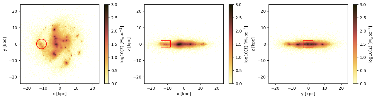
Cylindrical Region: Cutout the data assigned to the object particles
Select the ranges of the cylinder in the unit "kpc", relative to the given center [13., 24., 24.]. The height refers to both z-directions from the plane.
part_subregion = subregion(particles, :cylinder,
radius=3.,
height=2.,
range_unit=:kpc,
center=[13.,:bc,:bc],
direction=:z);[Mera]: 2025-06-30T20:24:26.016
center: [0.2708333, 0.5, 0.5] ==> [13.0 [kpc] :: 24.0 [kpc] :: 24.0 [kpc]]
domain:
xmin::xmax: 0.2083333 :: 0.3333333 ==> 10.0 [kpc] :: 16.0 [kpc]
ymin::ymax: 0.4375 :: 0.5625 ==> 21.0 [kpc] :: 27.0 [kpc]
zmin::zmax: 0.4583333 :: 0.5416667 ==> 22.0 [kpc] :: 26.0 [kpc]
Radius: 3.0 [kpc]
Height: 2.0 [kpc]
Memory used for data table :578.865234375 KB
-------------------------------------------------------Cylindrical Region: Projections of the sub-region.
The coordinates center is the center of the box:
proj_z = projection(part_subregion, :sd, unit=:Msol_pc2, center=[:boxcenter], direction=:z, lmax=10, verbose=false);
proj_y = projection(part_subregion, :sd, unit=:Msol_pc2, center=[:boxcenter], direction=:y, lmax=10, verbose=false);
proj_x = projection(part_subregion, :sd, unit=:Msol_pc2, center=[:boxcenter], direction=:x, lmax=10, verbose=false);figure(figsize=(15.5, 3.5))
labeltext = L"\mathrm{log10(\Sigma) \ [M_{\odot} pc^{-2}]}"
theta = range(-pi, stop=pi, length=100)
subplot(1,3,1)
im = imshow( log10.( permutedims(proj_z.maps[:sd]) ), cmap=cmap, aspect=proj_z.ratio, origin="lower", extent=proj_z.cextent, vmin=0, vmax=3)
plot( 3. .* sin.(theta) .-11, 3 .* cos.(theta), color="red")
xlabel("x [kpc]")
ylabel("y [kpc]")
cb = colorbar(im, label=labeltext)
subplot(1,3,2)
im = imshow( log10.( permutedims(proj_y.maps[:sd]) ), cmap=cmap, origin="lower", extent=proj_y.cextent, vmin=0, vmax=3)
xlabel("x [kpc]")
ylabel("z [kpc]")
cb = colorbar(im, orientation="horizontal", label=labeltext, pad=0.2);
subplot(1,3,3)
im = imshow( log10.( permutedims(proj_x.maps[:sd]) ), cmap=cmap, origin="lower", extent=proj_x.cextent, vmin=0, vmax=3)
xlabel("y [kpc]")
ylabel("z [kpc]")
cb = colorbar(im, orientation="horizontal", label=labeltext, pad=0.2);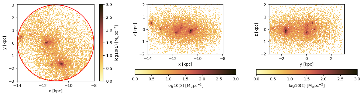
Cylindrical Region: Projections of the sub-region py passing a different center:
proj_z = projection(part_subregion, :sd, unit=:Msol_pc2, direction=:z, center=[13., 24.,24.], range_unit=:kpc, lmax=10, verbose=false);
proj_y = projection(part_subregion, :sd, unit=:Msol_pc2, direction=:y, center=[13., 24.,24.], range_unit=:kpc, lmax=10, verbose=false);
proj_x = projection(part_subregion, :sd, unit=:Msol_pc2, direction=:x, center=[13., 24.,24.], range_unit=:kpc, lmax=10, verbose=false);The ranges of the plots are now adapted to the given data center:
figure(figsize=(15.5, 3.5))
labeltext=L"\mathrm{log10(\Sigma) \ [M_{\odot} pc^{-2}]}"
theta = range(-pi, stop=pi, length=100)
subplot(1,3,1)
im = imshow( log10.( permutedims(proj_z.maps[:sd]) ), cmap=cmap, aspect=proj_z.ratio, origin="lower", extent=proj_z.cextent, vmin=0, vmax=3)
plot( 3. .* sin.(theta), 3 .* cos.(theta), color="red")
xlabel("x [kpc]")
ylabel("y [kpc]")
cb = colorbar(im, label=labeltext)
subplot(1,3,2)
im = imshow( log10.( permutedims(proj_y.maps[:sd]) ), cmap=cmap, origin="lower", extent=proj_y.cextent, vmin=0, vmax=3)
xlabel("x [kpc]")
ylabel("z [kpc]")
cb = colorbar(im, orientation="horizontal", label=labeltext, pad=0.2);
subplot(1,3,3)
im = imshow( log10.( permutedims(proj_x.maps[:sd]) ), cmap=cmap, origin="lower", extent=proj_x.cextent, vmin=0, vmax=3)
xlabel("y [kpc]")
ylabel("z [kpc]")
cb = colorbar(im, orientation="horizontal", label=labeltext, pad=0.2);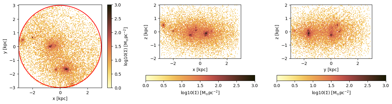
Cylindrical Region: Get the data outside of the selected region (inverse selection):
part_subregion = subregion(particles, :cylinder,
radius=3.,
height=2.,
range_unit=:kpc,
center=[ (24. -11.),:bc,:bc],
direction=:z,
inverse=true);[Mera]: 2025-06-30T20:24:26.678
center: [0.2708333, 0.5, 0.5] ==> [13.0 [kpc] :: 24.0 [kpc] :: 24.0 [kpc]]
domain:
xmin::xmax: 0.2083333 :: 0.3333333 ==> 10.0 [kpc] :: 16.0 [kpc]
ymin::ymax: 0.4375 :: 0.5625 ==> 21.0 [kpc] :: 27.0 [kpc]
zmin::zmax: 0.4583333 :: 0.5416667 ==> 22.0 [kpc] :: 26.0 [kpc]
Radius: 3.0 [kpc]
Height: 2.0 [kpc]
Memory used for data table :18.850629806518555 MB
-------------------------------------------------------proj_z = projection(part_subregion, :sd, unit=:Msol_pc2, center=[:boxcenter], direction=:z, lmax=8, verbose=false);
proj_y = projection(part_subregion, :sd, unit=:Msol_pc2, center=[:boxcenter], direction=:y, lmax=8, verbose=false);
proj_x = projection(part_subregion, :sd, unit=:Msol_pc2, center=[:boxcenter], direction=:x, lmax=8, verbose=false);figure(figsize=(15.5, 3.5))
labeltext=L"\mathrm{log10(\Sigma) \ [M_{\odot} pc^{-2}]}"
theta = range(-pi, stop=pi, length=100)
subplot(1,3,1)
im = imshow( log10.( permutedims(proj_z.maps[:sd]) ), cmap=cmap, aspect=proj_z.ratio, origin="lower", extent=proj_z.cextent, vmin=0, vmax=3)
plot( 3. .* sin.(theta) .-11, 3 .* cos.(theta), color="red")
xlabel("x [kpc]")
ylabel("y [kpc]")
cb = colorbar(im, label=labeltext)
subplot(1,3,2)
im = imshow( log10.( permutedims(proj_y.maps[:sd]) ), cmap=cmap, aspect=proj_y.ratio, origin="lower", extent=proj_y.cextent, vmin=0, vmax=3)
plot([-3.,3.,3.,-3.,-3.] .-11.,[-2.,-2.,2.,2.,-2.], color="red")
xlabel("x [kpc]")
ylabel("z [kpc]")
cb = colorbar(im, label=labeltext)
subplot(1,3,3)
im = imshow( log10.( permutedims(proj_x.maps[:sd]) ), cmap=cmap, aspect=proj_x.ratio, origin="lower", extent=proj_x.cextent, vmin=0, vmax=3)
plot([-3.,3.,3.,-3.,-3.],[-2.,-2.,2.,2.,-2.], color="red")
xlabel("y [kpc]")
ylabel("z [kpc]")
cb = colorbar(im, label=labeltext);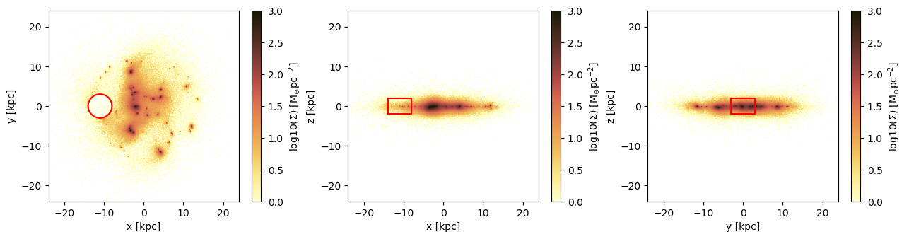
Spherical Region
Create projections of the full box:
proj_z = projection(particles, :sd, unit=:Msol_pc2, center=[:boxcenter], direction=:z, lmax=8, verbose=false);
proj_y = projection(particles, :sd, unit=:Msol_pc2, center=[:boxcenter], direction=:y, lmax=8, verbose=false);
proj_x = projection(particles, :sd, unit=:Msol_pc2, center=[:boxcenter], direction=:x, lmax=8, verbose=false);Spherical Region: The red lines show the region that we want to cutout as a sub-region from the full data:
figure(figsize=(15.5, 3.5))
labeltext=L"\mathrm{log10(\Sigma) \ [M_{\odot} pc^{-2}]}"
theta = range(-pi, stop=pi, length=100)
subplot(1,3,1)
im = imshow( log10.( permutedims(proj_z.maps[:sd]) ), cmap=cmap, aspect=proj_z.ratio, origin="lower", extent=proj_z.cextent, vmin=0, vmax=3)
plot( 10. .* sin.(theta) .-11., 10 .* cos.(theta), color="red")
xlabel("x [kpc]")
ylabel("y [kpc]")
cb = colorbar(im, label=labeltext)
subplot(1,3,2)
im = imshow( log10.( permutedims(proj_y.maps[:sd]) ), cmap=cmap, aspect=proj_y.ratio, origin="lower", extent=proj_y.cextent, vmin=0, vmax=3)
plot( 10. .* sin.(theta) .-11., 10 .* cos.(theta), color="red")
xlabel("x [kpc]")
ylabel("z [kpc]")
cb = colorbar(im, label=labeltext)
subplot(1,3,3)
im = imshow( log10.( permutedims(proj_x.maps[:sd]) ), cmap=cmap, aspect=proj_x.ratio, origin="lower", extent=proj_x.cextent, vmin=0, vmax=3)
plot( 10. .* sin.(theta) , 10 .* cos.(theta), color="red")
xlabel("y [kpc]")
ylabel("z [kpc]")
cb = colorbar(im, label=labeltext);
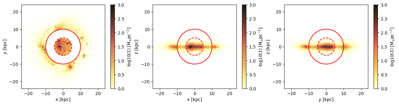
Spherical Region: Cutout the data assigned to the object particles
Select the radius of the sphere in the unit "kpc", relative to the given center [13., 24., 24.]:
part_subregion = subregion( particles, :sphere,
radius=10.,
range_unit=:kpc,
center=[(24. -11.),24.,24.]);[Mera]: 2025-06-30T20:24:27.501
center: [0.2708333, 0.5, 0.5] ==> [13.0 [kpc] :: 24.0 [kpc] :: 24.0 [kpc]]
domain:
xmin::xmax: 0.0625 :: 0.4791667 ==> 3.0 [kpc] :: 23.0 [kpc]
ymin::ymax: 0.2916667 :: 0.7083333 ==> 14.0 [kpc] :: 34.0 [kpc]
zmin::zmax: 0.2916667 :: 0.7083333 ==> 14.0 [kpc] :: 34.0 [kpc]
Radius: 10.0 [kpc]
Memory used for data table :8.807867050170898 MB
-------------------------------------------------------Spherical Region: Projections of the sub-region.
The coordinates center is the center of the box:
proj_z = projection(part_subregion, :sd, unit=:Msol_pc2, center=[:boxcenter], direction=:z, lmax=8, verbose=false);
proj_y = projection(part_subregion, :sd, unit=:Msol_pc2, center=[:boxcenter], direction=:y, lmax=8, verbose=false);
proj_x = projection(part_subregion, :sd, unit=:Msol_pc2, center=[:boxcenter], direction=:x, lmax=8, verbose=false);
figure(figsize=(15.5, 3.5))
labeltext=L"\mathrm{log10(\Sigma) \ [M_{\odot} pc^{-2}]}"
theta = range(-pi, stop=pi, length=100)
subplot(1,3,1)
im = imshow( log10.( permutedims(proj_z.maps[:sd]) ), cmap=cmap, aspect=proj_z.ratio, origin="lower", extent=proj_z.cextent, vmin=0, vmax=3)
plot( 10. .* sin.(theta) .-11., 10 .* cos.(theta), color="red")
xlabel("x [kpc]")
ylabel("y [kpc]")
cb = colorbar(im, label=labeltext)
subplot(1,3,2)
im = imshow( log10.( permutedims(proj_y.maps[:sd]) ), cmap=cmap, aspect=proj_y.ratio, origin="lower", extent=proj_y.cextent, vmin=0, vmax=3)
plot( 10. .* sin.(theta) .-11., 10 .* cos.(theta), color="red")
xlabel("x [kpc]")
ylabel("z [kpc]")
cb = colorbar(im, label=labeltext)
subplot(1,3,3)
im = imshow( log10.( permutedims(proj_x.maps[:sd]) ), cmap=cmap, aspect=proj_x.ratio, origin="lower", extent=proj_x.cextent, vmin=0, vmax=3)
plot( 10. .* sin.(theta) , 10 .* cos.(theta), color="red")
xlabel("y [kpc]")
ylabel("z [kpc]")
cb = colorbar(im, label=labeltext);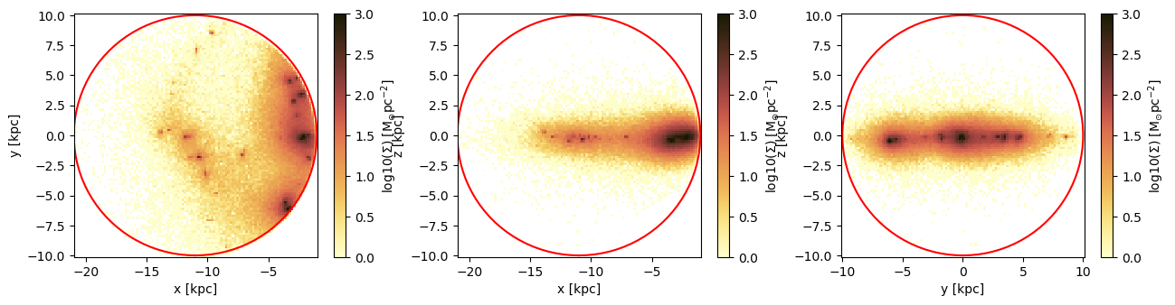
Spherical Region: Get the data outside of the selected region (inverse selection):
part_subregion = subregion( particles, :sphere,
radius=10.,
range_unit=:kpc,
center=[(24. -11.),24.,24.],
inverse=true);[Mera]: 2025-06-30T20:24:27.882
center: [0.2708333, 0.5, 0.5] ==> [13.0 [kpc] :: 24.0 [kpc] :: 24.0 [kpc]]
domain:
xmin::xmax: 0.0625 :: 0.4791667 ==> 3.0 [kpc] :: 23.0 [kpc]
ymin::ymax: 0.2916667 :: 0.7083333 ==> 14.0 [kpc] :: 34.0 [kpc]
zmin::zmax: 0.2916667 :: 0.7083333 ==> 14.0 [kpc] :: 34.0 [kpc]
Radius: 10.0 [kpc]
Memory used for data table :10.608060836791992 MB
-------------------------------------------------------proj_z = projection(part_subregion, :sd, unit=:Msol_pc2, center=[:boxcenter], direction=:z, lmax=8, verbose=false);
proj_y = projection(part_subregion, :sd, unit=:Msol_pc2, center=[:boxcenter], direction=:y, lmax=8, verbose=false);
proj_x = projection(part_subregion, :sd, unit=:Msol_pc2, center=[:boxcenter], direction=:x, lmax=8, verbose=false);figure(figsize=(15.5, 3.5))
labeltext=L"\mathrm{log10(\Sigma) \ [M_{\odot} pc^{-2}]}"
theta = range(-pi, stop=pi, length=100)
subplot(1,3,1)
im = imshow( log10.( permutedims(proj_z.maps[:sd]) ), cmap=cmap, aspect=proj_z.ratio, origin="lower", extent=proj_z.cextent, vmin=0, vmax=3)
plot( 10. .* sin.(theta) .-11., 10 .* cos.(theta), color="red")
xlabel("x [kpc]")
ylabel("y [kpc]")
cb = colorbar(im, label=labeltext)
subplot(1,3,2)
im = imshow( log10.( permutedims(proj_y.maps[:sd]) ), cmap=cmap, aspect=proj_y.ratio, origin="lower", extent=proj_y.cextent, vmin=0, vmax=3)
plot( 10. .* sin.(theta) .-11., 10 .* cos.(theta), color="red")
xlabel("x [kpc]")
ylabel("z [kpc]")
cb = colorbar(im, label=labeltext)
subplot(1,3,3)
im = imshow( log10.( permutedims(proj_x.maps[:sd]) ), cmap=cmap, aspect=proj_x.ratio, origin="lower", extent=proj_x.cextent, vmin=0, vmax=3)
plot( 10. .* sin.(theta) , 10 .* cos.(theta), color="red")
xlabel("y [kpc]")
ylabel("z [kpc]")
cb = colorbar(im, label=labeltext);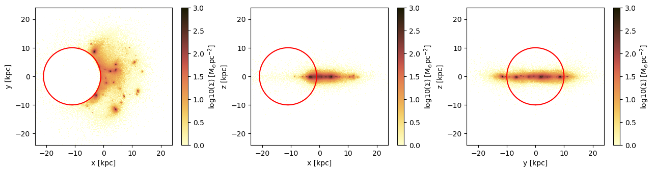
Combined/Nested/Shell Sub-Regions
The sub-region and shell functions can be used in any combination with each other! (Combined with overlapping ranges or nested)
One Example:
comb_region = subregion(particles, :cuboid, xrange=[-8.,8.], yrange=[-8.,8.], zrange=[-2.,2.], center=[:boxcenter], range_unit=:kpc, verbose=false)
comb_region2 = subregion(comb_region, :sphere, radius=12., center=[40.,24.,24.], range_unit=:kpc, inverse=true, verbose=false)
comb_region3 = subregion(comb_region2, :sphere, radius=12., center=[8.,24.,24.], range_unit=:kpc, inverse=true, verbose=false);
comb_region4 = subregion(comb_region3, :sphere, radius=12., center=[24.,5.,24.], range_unit=:kpc, inverse=true, verbose=false);
comb_region5 = subregion(comb_region4, :sphere, radius=12., center=[24.,43.,24.], range_unit=:kpc, inverse=true, verbose=false);proj_z = projection(comb_region5, :sd, unit=:Msol_pc2, lmax=8, center=[:boxcenter],direction=:z, verbose=false);
proj_y = projection(comb_region5, :sd, unit=:Msol_pc2, lmax=8, center=[:boxcenter],direction=:y, verbose=false);
proj_x = projection(comb_region5, :sd, unit=:Msol_pc2, lmax=8, center=[:boxcenter],direction=:x, verbose=false);figure(figsize=(15.5, 3.5))
labeltext=L"\mathrm{log10(\Sigma) \ [M_{\odot} pc^{-2}]}"
subplot(1,3,1)
im = imshow( log10.(permutedims(proj_z.maps[:sd]) ), cmap=cmap, aspect=proj_z.ratio, origin="lower")#, extent=proj_z.cextent, vmin=0, vmax=3)
xlabel("x [kpc]")
ylabel("y [kpc]")
cb = colorbar(im, label=labeltext)
subplot(1,3,2)
im = imshow( log10.(permutedims(proj_y.maps[:sd]) ), cmap=cmap, origin="lower") #, extent=proj_y.cextent, vmin=0, vmax=3)
xlabel("x [kpc]")
ylabel("z [kpc]")
cb = colorbar(im, label=labeltext)
subplot(1,3,3)
im = imshow( log10.(permutedims(proj_x.maps[:sd]) ), cmap=cmap, origin="lower")#, extent=proj_x.cextent, vmin=0, vmax=3)
xlabel("y [kpc]")
ylabel("z [kpc]")
cb = colorbar(im, label=labeltext);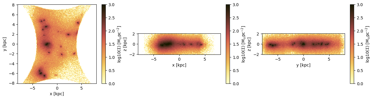
Cylindrical Shell
Create projections of the full box:
proj_z = projection(particles, :sd, unit=:Msol_pc2, center=[:boxcenter], direction=:z, lmax=8, verbose=false);
proj_y = projection(particles, :sd, unit=:Msol_pc2, center=[:boxcenter], direction=:y, lmax=8, verbose=false);
proj_x = projection(particles, :sd, unit=:Msol_pc2, center=[:boxcenter], direction=:x, lmax=8, verbose=false);
Cylindrical Shell: The red lines show the shell we want to cutout as a sub-region from the full data:
figure(figsize=(15.5, 3.5))
labeltext=L"\mathrm{log10(\Sigma) \ [M_{\odot} pc^{-2}]}"
theta = range(-pi, stop=pi, length=100)
subplot(1,3,1)
im = imshow( log10.( permutedims(proj_z.maps[:sd]) ), cmap=cmap, aspect=proj_z.ratio, origin="lower", extent=proj_z.cextent, vmin=0, vmax=3)
plot( 10. .* sin.(theta) , 10 .* cos.(theta), color="red")
plot( 5. .* sin.(theta) , 5. .* cos.(theta), color="red", ls="--")
xlabel("x [kpc]")
ylabel("y [kpc]")
cb = colorbar(im, label=labeltext)
subplot(1,3,2)
im = imshow( log10.( permutedims(proj_y.maps[:sd]) ), cmap=cmap, aspect=proj_y.ratio, origin="lower", extent=proj_y.cextent, vmin=0, vmax=3)
plot([-10.,-10.,10.,10.,-10.], [-2.,2.,2.,-2.,-2.], color="red")
plot([-5.,-5,5.,5.,-5.], [-2.,2.,2.,-2.,-2.], color="red", ls="--")
xlabel("x [kpc]")
ylabel("z [kpc]")
cb = colorbar(im, label=labeltext)
subplot(1,3,3)
im = imshow( log10.(permutedims(proj_x.maps[:sd]) ), cmap=cmap, aspect=proj_x.ratio, origin="lower", extent=proj_x.cextent, vmin=0, vmax=3)
plot([-10.,-10.,10.,10.,-10.], [-2.,2.,2.,-2.,-2.], color="red")
plot([-5.,-5,5.,5.,-5.], [-2.,2.,2.,-2.,-2.], color="red", ls="--")
xlabel("y [kpc]")
ylabel("z [kpc]")
cb = colorbar(im, label=labeltext);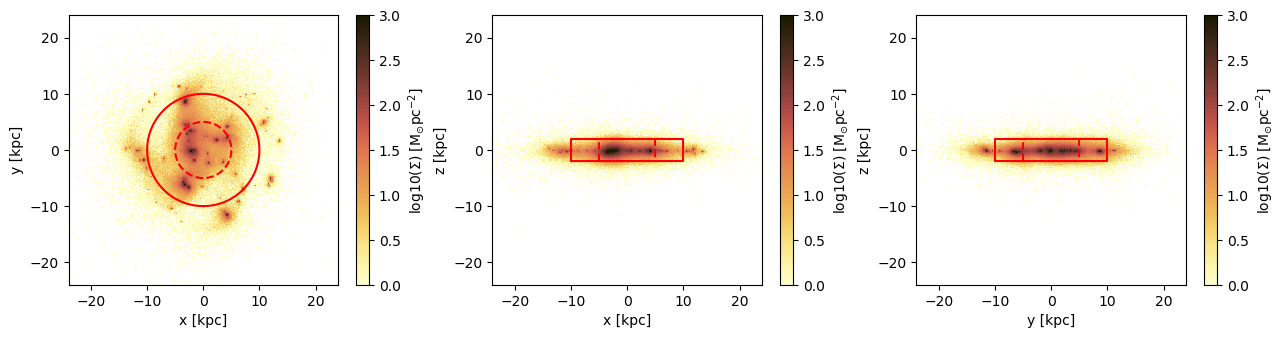
Cylindrical Shell:
Pass the height of the cylinder and the inner/outer radius of the shell in the unit "kpc", relative to the box center [24., 24., 24.]:
part_subregion = shellregion( particles, :cylinder,
radius=[5.,10.],
height=2.,
range_unit=:kpc,
center=[:boxcenter]);[Mera]: 2025-06-30T20:24:29.363
center: [0.5, 0.5, 0.5] ==> [24.0 [kpc] :: 24.0 [kpc] :: 24.0 [kpc]]
domain:
xmin::xmax: 0.2916667 :: 0.7083333 ==> 14.0 [kpc] :: 34.0 [kpc]
ymin::ymax: 0.2916667 :: 0.7083333 ==> 14.0 [kpc] :: 34.0 [kpc]
zmin::zmax: 0.4583333 :: 0.5416667 ==> 22.0 [kpc] :: 26.0 [kpc]
Inner radius: 5.0 [kpc]
Outer radius: 10.0 [kpc]
Radius diff: 5.0 [kpc]
Height: 2.0 [kpc]
Memory used for data table :7.282751083374023 MB
-------------------------------------------------------proj_z = projection(part_subregion, :sd, unit=:Msol_pc2, center=[:boxcenter], direction=:z, lmax=8, verbose=false);
proj_y = projection(part_subregion, :sd, unit=:Msol_pc2, center=[:boxcenter], direction=:y, lmax=8, verbose=false);
proj_x = projection(part_subregion, :sd, unit=:Msol_pc2, center=[:boxcenter], direction=:x, lmax=8, verbose=false);figure(figsize=(15.5, 3.5))
labeltext=L"\mathrm{log10(\Sigma) \ [M_{\odot} pc^{-2}]}"
theta = range(-pi, stop=pi, length=100)
subplot(1,3,1)
im = imshow( log10.( permutedims(proj_z.maps[:sd]) ), cmap=cmap, aspect=proj_z.ratio, origin="lower", extent=proj_z.cextent, vmin=0, vmax=3)
plot( 10. .* sin.(theta) , 10 .* cos.(theta), color="red")
plot( 5. .* sin.(theta) , 5. .* cos.(theta), color="red", ls="--")
xlabel("x [kpc]")
ylabel("y [kpc]")
cb = colorbar(im, label=labeltext)
subplot(1,3,2)
im = imshow( log10.( permutedims(proj_y.maps[:sd]) ), cmap=cmap, origin="lower", extent=proj_y.cextent, vmin=0, vmax=3)
plot([-10.,-10.,10.,10.,-10.], [-2.,2.,2.,-2.,-2.], color="red")
plot([-5.,-5,5.,5.,-5.], [-2.,2.,2.,-2.,-2.], color="red", ls="--")
xlabel("x [kpc]")
ylabel("z [kpc]")
cb = colorbar(im, orientation="horizontal", label=labeltext, pad=0.2);
subplot(1,3,3)
im = imshow( log10.( permutedims(proj_x.maps[:sd]) ), cmap=cmap, origin="lower", extent=proj_x.cextent, vmin=0, vmax=3)
plot([-10.,-10.,10.,10.,-10.], [-2.,2.,2.,-2.,-2.], color="red")
plot([-5.,-5,5.,5.,-5.], [-2.,2.,2.,-2.,-2.], color="red", ls="--")
xlabel("y [kpc]")
ylabel("z [kpc]")
cb = colorbar(im, orientation="horizontal", label=labeltext, pad=0.2);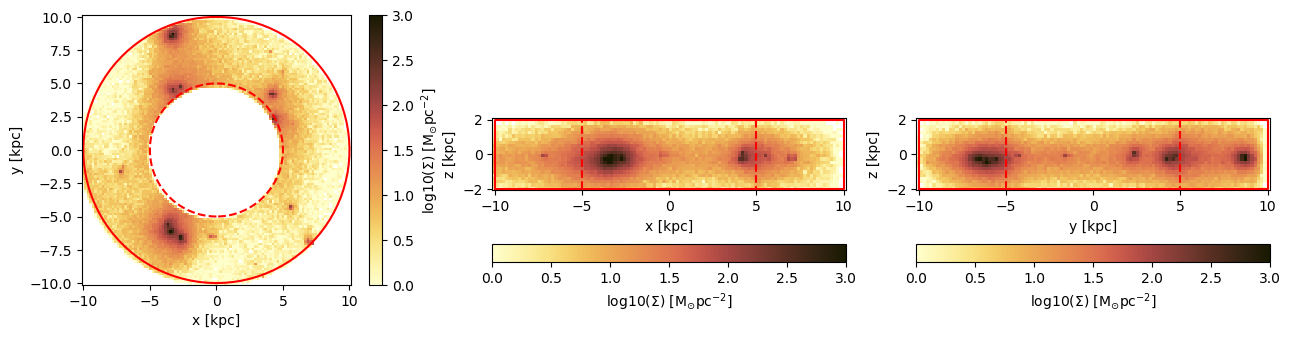
Cylindrical Shell: Get the data outside of the selected shell (inverse selection):
part_subregion = shellregion( particles, :cylinder,
radius=[5.,10.],
height=2.,
range_unit=:kpc,
center=[:boxcenter],
inverse=true);[Mera]: 2025-06-30T20:24:29.804
center: [0.5, 0.5, 0.5] ==> [24.0 [kpc] :: 24.0 [kpc] :: 24.0 [kpc]]
domain:
xmin::xmax: 0.2916667 :: 0.7083333 ==> 14.0 [kpc] :: 34.0 [kpc]
ymin::ymax: 0.2916667 :: 0.7083333 ==> 14.0 [kpc] :: 34.0 [kpc]
zmin::zmax: 0.4583333 :: 0.5416667 ==> 22.0 [kpc] :: 26.0 [kpc]
Inner radius: 5.0 [kpc]
Outer radius: 10.0 [kpc]
Radius diff: 5.0 [kpc]
Height: 2.0 [kpc]
Memory used for data table :12.133176803588867 MB
-------------------------------------------------------proj_z = projection(part_subregion, :sd, unit=:Msol_pc2, center=[:boxcenter], direction=:z, lmax=8, verbose=false);
proj_y = projection(part_subregion, :sd, unit=:Msol_pc2, center=[:boxcenter], direction=:y, lmax=8, verbose=false);
proj_x = projection(part_subregion, :sd, unit=:Msol_pc2, center=[:boxcenter], direction=:x, lmax=8, verbose=false);figure(figsize=(15.5, 3.5))
labeltext=L"\mathrm{log10(\Sigma) \ [M_{\odot} pc^{-2}]}"
theta = range(-pi, stop=pi, length=100)
subplot(1,3,1)
im = imshow( log10.( permutedims(proj_z.maps[:sd]) ), cmap=cmap, aspect=proj_z.ratio, origin="lower", extent=proj_z.cextent, vmin=0, vmax=3)
plot( 10. .* sin.(theta) , 10 .* cos.(theta), color="red")
plot( 5. .* sin.(theta) , 5. .* cos.(theta), color="red", ls="--")
xlabel("x [kpc]")
ylabel("y [kpc]")
cb = colorbar(im, label=labeltext)
subplot(1,3,2)
im = imshow( log10.( permutedims(proj_y.maps[:sd]) ), cmap=cmap, aspect=proj_y.ratio, origin="lower", extent=proj_y.cextent, vmin=0, vmax=3)
plot([-10.,-10.,10.,10.,-10.], [-2.,2.,2.,-2.,-2.], color="red")
plot([-5.,-5,5.,5.,-5.], [-2.,2.,2.,-2.,-2.], color="red", ls="--")
xlabel("x [kpc]")
ylabel("z [kpc]")
cb = colorbar(im, label=labeltext)
subplot(1,3,3)
im = imshow( log10.( permutedims(proj_x.maps[:sd]) ), cmap=cmap, aspect=proj_x.ratio, origin="lower", extent=proj_x.cextent, vmin=0, vmax=3)
plot([-10.,-10.,10.,10.,-10.], [-2.,2.,2.,-2.,-2.], color="red")
plot([-5.,-5,5.,5.,-5.], [-2.,2.,2.,-2.,-2.], color="red", ls="--")
xlabel("y [kpc]")
ylabel("z [kpc]")
cb = colorbar(im, label=labeltext);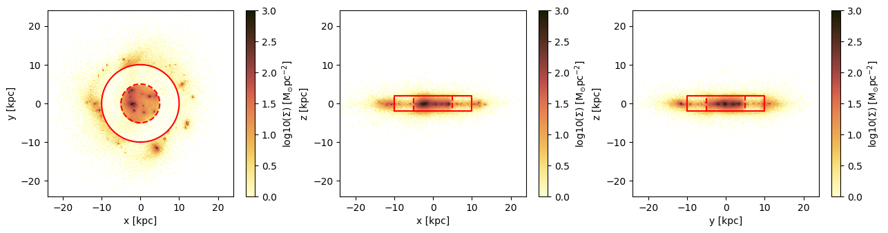
<a id="ShellRegionSphere"></a>
Spherical Shell
Create projections of the full box:
proj_z = projection(particles, :sd, unit=:Msol_pc2, center=[:boxcenter], direction=:z, lmax=8, verbose=false);
proj_y = projection(particles, :sd, unit=:Msol_pc2, center=[:boxcenter], direction=:y, lmax=8, verbose=false);
proj_x = projection(particles, :sd, unit=:Msol_pc2, center=[:boxcenter], direction=:x, lmax=8, verbose=false);Spherical Shell: The red lines show the shell that we want to cutout as a sub-region from the full data:
figure(figsize=(15.5, 3.5))
labeltext=L"\mathrm{log10(\Sigma) \ [M_{\odot} pc^{-2}]}"
theta = range(-pi, stop=pi, length=100)
subplot(1,3,1)
im = imshow( log10.( permutedims(proj_z.maps[:sd]) ), cmap=cmap, aspect=proj_z.ratio, origin="lower", extent=proj_z.cextent, vmin=0, vmax=3)
plot( 10. .* sin.(theta) , 10 .* cos.(theta), color="red")
plot( 5. .* sin.(theta) , 5. .* cos.(theta), color="red", ls="--")
xlabel("x [kpc]")
ylabel("y [kpc]")
cb = colorbar(im, label=labeltext)
subplot(1,3,2)
im = imshow( log10.( permutedims(proj_y.maps[:sd]) ), cmap=cmap, aspect=proj_y.ratio, origin="lower", extent=proj_y.cextent, vmin=0, vmax=3)
plot( 10. .* sin.(theta) , 10 .* cos.(theta), color="red")
plot( 5. .* sin.(theta) , 5. .* cos.(theta), color="red", ls="--")
xlabel("x [kpc]")
ylabel("z [kpc]")
cb = colorbar(im, label=labeltext)
subplot(1,3,3)
im = imshow( log10.( permutedims(proj_x.maps[:sd]) ), cmap=cmap, aspect=proj_x.ratio, origin="lower", extent=proj_x.cextent, vmin=0, vmax=3)
plot( 10. .* sin.(theta) , 10 .* cos.(theta), color="red")
plot( 5. .* sin.(theta) , 5. .* cos.(theta), color="red",ls="--")
xlabel("y [kpc]")
ylabel("z [kpc]")
cb = colorbar(im, label=labeltext);
Spherical Shell:
Select the inner and outer radius of the spherical shell in unit "kpc", relative to the box center [24., 24., 24.]:
part_subregion = shellregion( particles, :sphere,
radius=[5.,10.],
range_unit=:kpc,
center=[24.,24.,24.]);[Mera]: 2025-06-30T20:24:30.864
center: [0.5, 0.5, 0.5] ==> [24.0 [kpc] :: 24.0 [kpc] :: 24.0 [kpc]]
domain:
xmin::xmax: 0.2916667 :: 0.7083333 ==> 14.0 [kpc] :: 34.0 [kpc]
ymin::ymax: 0.2916667 :: 0.7083333 ==> 14.0 [kpc] :: 34.0 [kpc]
zmin::zmax: 0.2916667 :: 0.7083333 ==> 14.0 [kpc] :: 34.0 [kpc]
Inner radius: 5.0 [kpc]
Outer radius: 10.0 [kpc]
Radius diff: 5.0 [kpc]
Memory used for data table :7.59193229675293 MB
-------------------------------------------------------Spherical Shell: Projections of the shell-region.
The coordinates center is the center of the box:
proj_z = projection(part_subregion, :sd, unit=:Msol_pc2, center=[:boxcenter], direction=:z, lmax=8, verbose=false);
proj_y = projection(part_subregion, :sd, unit=:Msol_pc2, center=[:boxcenter], direction=:y, lmax=8, verbose=false);
proj_x = projection(part_subregion, :sd, unit=:Msol_pc2, center=[:boxcenter], direction=:x, lmax=8, verbose=false);
figure(figsize=(15.5, 3.5))
labeltext=L"\mathrm{log10(\Sigma) \ [M_{\odot} pc^{-2}]}"
theta = range(-pi, stop=pi, length=100)
subplot(1,3,1)
im = imshow( log10.( permutedims(proj_z.maps[:sd]) ), cmap=cmap, aspect=proj_z.ratio, origin="lower", extent=proj_z.cextent, vmin=0, vmax=3)
plot( 10. .* sin.(theta) , 10 .* cos.(theta), color="red")
plot( 5. .* sin.(theta) , 5. .* cos.(theta), color="red", ls="--")
xlabel("x [kpc]")
ylabel("y [kpc]")
cb = colorbar(im, label=labeltext)
subplot(1,3,2)
im = imshow( log10.( permutedims(proj_y.maps[:sd]) ), cmap=cmap, aspect=proj_y.ratio, origin="lower", extent=proj_y.cextent, vmin=0, vmax=3)
plot( 10. .* sin.(theta) , 10 .* cos.(theta), color="red")
plot( 5. .* sin.(theta) , 5. .* cos.(theta), color="red",ls="--")
xlabel("x [kpc]")
ylabel("z [kpc]")
cb = colorbar(im, label=labeltext);
subplot(1,3,3)
im = imshow( log10.( permutedims(proj_x.maps[:sd]) ), cmap=cmap, aspect=proj_x.ratio, origin="lower", extent=proj_x.cextent, vmin=0, vmax=3)
plot( 10. .* sin.(theta) , 10 .* cos.(theta), color="red")
plot( 5. .* sin.(theta) , 5. .* cos.(theta), color="red",ls="--")
xlabel("y [kpc]")
ylabel("z [kpc]")
cb = colorbar(im, label=labeltext);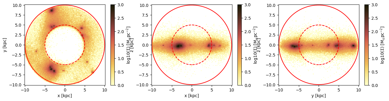
Spherical Shell: Get the data outside of the selected shell-region (inverse selection):
part_subregion = shellregion( particles, :sphere,
                                radius=[5.,10.],
                                range_unit=:kpc,
                                center=[:boxcenter],
inverse=true);[Mera]: 2025-06-30T20:24:31.433
center: [0.5, 0.5, 0.5] ==> [24.0 [kpc] :: 24.0 [kpc] :: 24.0 [kpc]]
domain:
xmin::xmax: 0.2916667 :: 0.7083333 ==> 14.0 [kpc] :: 34.0 [kpc]
ymin::ymax: 0.2916667 :: 0.7083333 ==> 14.0 [kpc] :: 34.0 [kpc]
zmin::zmax: 0.2916667 :: 0.7083333 ==> 14.0 [kpc] :: 34.0 [kpc]
Inner radius: 5.0 [kpc]
Outer radius: 10.0 [kpc]
Radius diff: 5.0 [kpc]
Memory used for data table :11.823995590209961 MB
-------------------------------------------------------proj_z = projection(part_subregion, :sd, unit=:Msol_pc2, center=[:boxcenter], direction=:z, lmax=8, verbose=false);
proj_y = projection(part_subregion, :sd, unit=:Msol_pc2, center=[:boxcenter], direction=:y, lmax=8, verbose=false);
proj_x = projection(part_subregion, :sd, unit=:Msol_pc2, center=[:boxcenter], direction=:x, lmax=8, verbose=false);figure(figsize=(15.5, 3.5))
labeltext=L"\mathrm{log10(\Sigma) \ [M_{\odot} pc^{-2}]}"
theta = range(-pi, stop=pi, length=100)
subplot(1,3,1)
im = imshow( log10.( permutedims(proj_z.maps[:sd]) ), cmap=cmap, aspect=proj_z.ratio, origin="lower", extent=proj_z.cextent, vmin=0, vmax=3)
plot( 10. .* sin.(theta) , 10 .* cos.(theta), color="red")
plot( 5. .* sin.(theta) , 5. .* cos.(theta), color="red", ls="--")
xlabel("x [kpc]")
ylabel("y [kpc]")
cb = colorbar(im, label=labeltext)
subplot(1,3,2)
im = imshow( log10.( permutedims(proj_y.maps[:sd]) ), cmap=cmap, aspect=proj_y.ratio, origin="lower", extent=proj_y.cextent, vmin=0, vmax=3)
plot( 10. .* sin.(theta) , 10 .* cos.(theta), color="red")
plot( 5. .* sin.(theta) , 5. .* cos.(theta), color="red", ls="--")
xlabel("x [kpc]")
ylabel("z [kpc]")
cb = colorbar(im, label=labeltext)
subplot(1,3,3)
im = imshow( log10.( permutedims(proj_x.maps[:sd]) ), cmap=cmap, aspect=proj_x.ratio, origin="lower", extent=proj_x.cextent, vmin=0, vmax=3)
plot( 10. .* sin.(theta) , 10 .* cos.(theta), color="red")
plot( 5. .* sin.(theta) , 5. .* cos.(theta), color="red", ls="--")
xlabel("y [kpc]")
ylabel("z [kpc]")
cb = colorbar(im, label=labeltext);