3. Hydro: Get Sub-Regions of The Loaded Data
Load the Data
using Mera, PyPlot
using ColorSchemes
cmap = ColorMap(ColorSchemes.lajolla.colors) # See http://www.fabiocrameri.ch/colourmaps.php

info = getinfo(400, "../../testing/simulations/manu_sim_sf_L14")
gas  = gethydro(info, :rho, lmax=10, smallr=1e-5);
[Mera]: 2020-02-18T23:23:22.753
Code: RAMSES
output [400] summary:
mtime: 2018-09-05T09:51:55.041
ctime: 2019-11-01T17:35:21.051
=======================================================
simulation time: 594.98 [Myr]
boxlen: 48.0 [kpc]
ncpu: 2048
ndim: 3
-------------------------------------------------------
amr: true
level(s): 6 - 14 --> cellsize(s): 750.0 [pc] - 2.93 [pc]
-------------------------------------------------------
hydro: true
hydro-variables: 7 --> (:rho, :vx, :vy, :vz, :p, :var6, :var7)
hydro-descriptor: (:density, :velocity_x, :velocity_y, :velocity_z, :thermal_pressure, :passive_scalar_1, :passive_scalar_2)
γ: 1.6667
-------------------------------------------------------
gravity: true
gravity-variables: (:epot, :ax, :ay, :az)
-------------------------------------------------------
particles: true
- Npart: 5.091500e+05
- Nstars: 5.066030e+05
- Ndm: 2.547000e+03
particle variables: (:vx, :vy, :vz, :mass, :birth)
-------------------------------------------------------
clumps: true
clump-variables: (:index, :lev, :parent, :ncell, :peak_x, :peak_y, :peak_z, Symbol("rho-"), Symbol("rho+"), :rho_av, :mass_cl, :relevance)
-------------------------------------------------------
namelist-file: false
timer-file: false
compilation-file: true
makefile: true
patchfile: true
=======================================================
[Mera]: Get hydro data: 2020-02-18T23:23:32.417
Key vars=(:level, :cx, :cy, :cz)
Using var(s)=(1,) = (:rho,)
domain:
xmin::xmax: 0.0 :: 1.0 ==> 0.0 [kpc] :: 48.0 [kpc]
ymin::ymax: 0.0 :: 1.0 ==> 0.0 [kpc] :: 48.0 [kpc]
zmin::zmax: 0.0 :: 1.0 ==> 0.0 [kpc] :: 48.0 [kpc]
Reading data...
100%|███████████████████████████████████████████████████| Time: 0:02:49
Memory used for data table :186.1558656692505 MB
-------------------------------------------------------Cuboid Region
Create projections of the full box:
proj_z = projection(gas, :sd, :Msol_pc2, center=[:boxcenter], direction=:z, verbose=false);
proj_y = projection(gas, :sd, :Msol_pc2, center=[:boxcenter], direction=:y, verbose=false);
proj_x = projection(gas, :sd, :Msol_pc2, center=[:boxcenter], direction=:x, verbose=false);
100%|███████████████████████████████████████████████████| Time: 0:00:03The generated objects include, e.g. the extent of the processed domain, that can be used to declare the specific range of the plots, while the field cextent gives the extent related to a given center (default: [0.,0.,0.]).
propertynames(proj_z)(:maps, :maps_unit, :maps_lmax, :maps_mode, :lmax_projected, :lmin, :lmax, :ranges, :extent, :cextent, :ratio, :boxlen, :smallr, :smallc, :scale, :info)Cuboid Region: The red lines show the region that we want to cutout as a sub-region from the full data:
figure(figsize=(15.5, 3.5))
labeltext = L"\mathrm{log10(\Sigma) \ [M_{\odot} pc^{-2}]}"

subplot(1,3,1)
im = imshow( log10.( permutedims(proj_z.maps[:sd]) ), cmap=cmap, aspect=proj_z.ratio, origin="lower", extent=proj_z.cextent, vmin=0, vmax=3)
plot([-4.,0.,0.,-4.,-4.],[-15.,-15.,15.,15.,-15.], color="red")
xlabel("x [kpc]")
ylabel("y [kpc]")
cb = colorbar(im, label=labeltext)

subplot(1,3,2)
im = imshow( log10.( permutedims(proj_y.maps[:sd]) ), cmap=cmap, aspect=proj_y.ratio, origin="lower", extent=proj_y.cextent, vmin=0, vmax=3)
plot([-4.,0.,0.,-4.,-4.],[-2.,-2.,2.,2.,-2.], color="red")
xlabel("x [kpc]")
ylabel("z [kpc]")
cb = colorbar(im, label=labeltext)

subplot(1,3,3)
im = imshow( log10.( permutedims(proj_x.maps[:sd]) ), cmap=cmap, aspect=proj_x.ratio, origin="lower", extent=proj_x.cextent, vmin=0, vmax=3)
plot([-15.,15.,15.,-15.,-15.],[-2.,-2.,2.,2.,-2.], color="red")
xlabel("y [kpc]")
ylabel("z [kpc]")
cb = colorbar(im, label=labeltext);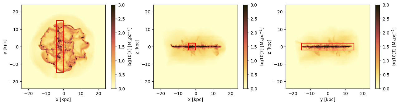
Cuboid Region: Cutout the data assigned to the object gas
Note: The selected regions can be given relative to a user given center or to the box corner [0., 0., 0.] by default. The user can choose between standard notation 0:1 or physical length-units, defined in e.g. info.scale :
gas_subregion = subregion( gas, :cuboid,
                            xrange=[-4., 0.],
                            yrange=[-15., 15.],
                            zrange=[-2., 2.],
                            center=[:boxcenter],
                            range_unit=:kpc);
[Mera]: 2020-02-18T23:27:06.861
center: [0.5, 0.5, 0.5] ==> [24.0 [kpc] :: 24.0 [kpc] :: 24.0 [kpc]]
domain:
xmin::xmax: 0.4166667 :: 0.5 ==> 20.0 [kpc] :: 24.0 [kpc]
ymin::ymax: 0.1875 :: 0.8125 ==> 9.0 [kpc] :: 39.0 [kpc]
zmin::zmax: 0.4583333 :: 0.5416667 ==> 22.0 [kpc] :: 26.0 [kpc]
Memory used for data table :47.87415790557861 MB
-------------------------------------------------------The function subregion creates a new object with the same type as the object created by the function gethydro :
typeof(gas_subregion)HydroDataTypeCuboid Region: Projections of the sub-region.
The coordinates center is the center of the box:
proj_z = projection(gas_subregion, :sd, :Msol_pc2, center=[:boxcenter], direction=:z, verbose=false);
proj_y = projection(gas_subregion, :sd, :Msol_pc2, center=[:boxcenter], direction=:y, verbose=false);
proj_x = projection(gas_subregion, :sd, :Msol_pc2, center=[:boxcenter], direction=:x, verbose=false);
figure(figsize=(15.5, 3.5))
labeltext = L"\mathrm{log10(\Sigma) \ [M_{\odot} pc^{-2}]}"
subplot(1,3,1)
im = imshow( log10.(permutedims(proj_z.maps[:sd]) ), cmap=cmap, origin="lower", extent=proj_z.cextent, vmin=0, vmax=3)
xlabel("x [kpc]")
ylabel("y [kpc]")
cb = colorbar(im, label=labeltext)
subplot(1,3,2)
im = imshow( log10.(permutedims(proj_y.maps[:sd]) ), cmap=cmap, origin="lower", extent=proj_y.cextent, vmin=0, vmax=3)
xlabel("x [kpc]")
ylabel("z [kpc]")
cb = colorbar(im, label=labeltext)
subplot(1,3,3)
im = imshow( log10.(permutedims(proj_x.maps[:sd]) ), cmap=cmap, origin="lower", extent=proj_x.cextent, vmin=0, vmax=3)
xlabel("y [kpc]")
ylabel("z [kpc]")
ylabel("z [kpc]")
cb = colorbar(im, orientation="horizontal", label=labeltext, pad=0.2);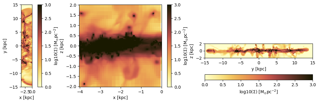
Cuboid Region: Get the data outside of the selected region (inverse selection):
gas_subregion = subregion( gas, :cuboid,
                            xrange=[-4., 0.],
                            yrange=[-15., 15.],
                            zrange=[-2., 2.],
                            center=[:boxcenter],
                            range_unit=:kpc,
                            inverse=true);
[Mera]: 2020-02-18T23:27:09.597
center: [0.5, 0.5, 0.5] ==> [24.0 [kpc] :: 24.0 [kpc] :: 24.0 [kpc]]
domain:
xmin::xmax: 0.4166667 :: 0.5 ==> 20.0 [kpc] :: 24.0 [kpc]
ymin::ymax: 0.1875 :: 0.8125 ==> 9.0 [kpc] :: 39.0 [kpc]
zmin::zmax: 0.4583333 :: 0.5416667 ==> 22.0 [kpc] :: 26.0 [kpc]
Memory used for data table :138.2824068069458 MB
-------------------------------------------------------proj_z = projection(gas_subregion, :sd, :Msol_pc2, center=[:boxcenter], direction=:z, verbose=false);
proj_y = projection(gas_subregion, :sd, :Msol_pc2, center=[:boxcenter], direction=:y, verbose=false);
proj_x = projection(gas_subregion, :sd, :Msol_pc2, center=[:boxcenter], direction=:x, verbose=false); 100%|███████████████████████████████████████████████████| Time: 0:00:01figure(figsize=(15.5, 3.5))
labeltext = L"\mathrm{log10(\Sigma) \ [M_{\odot} pc^{-2}]}"
subplot(1,3,1)
im = imshow( log10.(permutedims(proj_z.maps[:sd]) ), cmap=cmap, aspect=proj_z.ratio, origin="lower", extent=proj_z.cextent, vmin=0, vmax=3)
plot([-4.,0.,0.,-4.,-4.],[-15.,-15.,15.,15.,-15.], color="red")
xlabel("x [kpc]")
ylabel("y [kpc]")
cb = colorbar(im, label=labeltext)
subplot(1,3,2)
im = imshow( log10.(permutedims(proj_y.maps[:sd]) ), cmap=cmap, aspect=proj_y.ratio, origin="lower", extent=proj_y.cextent, vmin=0, vmax=3)
plot([-4.,0.,0.,-4.,-4.],[-2.,-2.,2.,2.,-2.], color="red")
xlabel("x [kpc]")
ylabel("z [kpc]")
cb = colorbar(im, label=labeltext)
subplot(1,3,3)
im = imshow( log10.(permutedims(proj_x.maps[:sd]) ), cmap=cmap, aspect=proj_x.ratio, origin="lower", extent=proj_x.cextent, vmin=0, vmax=3)
plot([-15.,15.,15.,-15.,-15.],[-2.,-2.,2.,2.,-2.], color="red")
xlabel("y [kpc]")
ylabel("z [kpc]")
cb = colorbar(im, label=labeltext);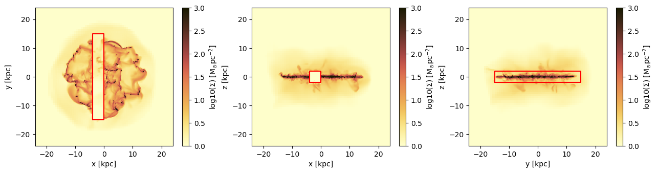
Cylindrical Region
Create projections of the full box:
proj_z = projection(gas, :sd, :Msol_pc2, center=[:boxcenter], direction=:z, verbose=false);
proj_y = projection(gas, :sd, :Msol_pc2, center=[:boxcenter], direction=:y, verbose=false);
proj_x = projection(gas, :sd, :Msol_pc2, center=[:boxcenter], direction=:x, verbose=false); 100%|███████████████████████████████████████████████████| Time: 0:00:01
100%|███████████████████████████████████████████████████| Time: 0:00:01Cylindrical Region: The red lines show the region that we want to cutout as a sub-region from the full data:
figure(figsize=(15.5, 3.5))
labeltext = L"\mathrm{log10(\Sigma) \ [M_{\odot} pc^{-2}]}"
theta = LinRange(-pi, pi, 100)
subplot(1,3,1)
im = imshow( log10.(permutedims(proj_z.maps[:sd]) ), cmap=cmap, aspect=proj_z.ratio, origin="lower", extent=proj_z.cextent, vmin=0, vmax=3)
plot( 3. .* sin.(theta) .-11, 3 .* cos.(theta), color="red")
xlabel("x [kpc]")
ylabel("y [kpc]")
cb = colorbar(im, label=labeltext)
subplot(1,3,2)
im = imshow( log10.(permutedims(proj_y.maps[:sd]) ), cmap=cmap, origin="lower", extent=proj_y.cextent, vmin=0, vmax=3)
plot([-3.,3.,3.,-3.,-3.] .-11.,[-2.,-2.,2.,2.,-2.], color="red")
xlabel("x [kpc]")
ylabel("z [kpc]")
cb = colorbar(im, label=labeltext)
subplot(1,3,3)
im = imshow( log10.(permutedims(proj_x.maps[:sd]) ), cmap=cmap, origin="lower", extent=proj_x.cextent, vmin=0, vmax=3)
plot([-3.,3.,3.,-3.,-3.],[-2.,-2.,2.,2.,-2.], color="red")
xlabel("y [kpc]")
ylabel("z [kpc]")
cb = colorbar(im, label=labeltext);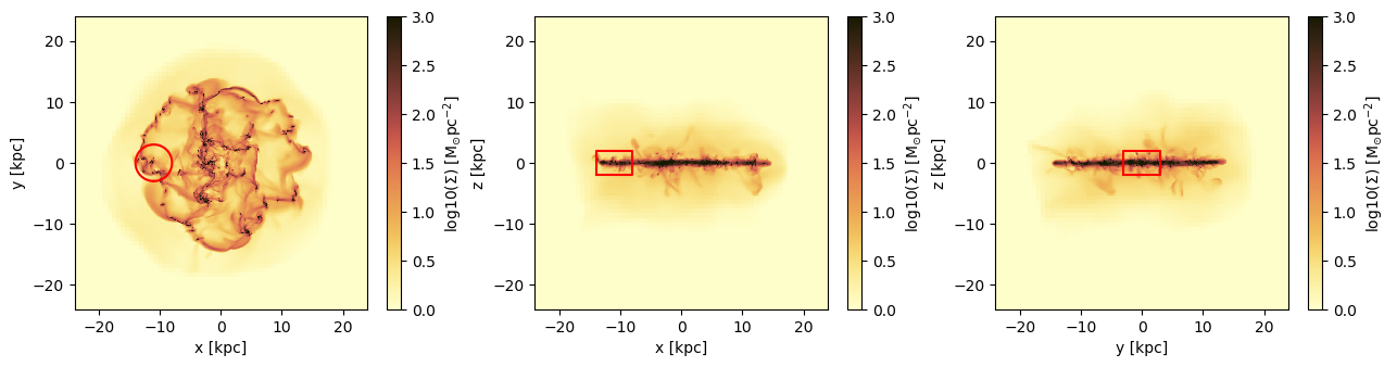
Cylindrical Region: Cutout the data assigned to the object gas
Select the ranges of the cylinder in the unit "kpc", relative to the given center [13., 24., 24.]. The height refers to both z-directions from the plane.
gas_subregion = subregion( gas, :cylinder,
radius=3.,
height=2.,
range_unit=:kpc,
center=[13., :bc, :bc]); # direction=:z, by default [Mera]: 2020-02-18T23:27:24.715
center: [0.2708333, 0.5, 0.5] ==> [13.0 [kpc] :: 24.0 [kpc] :: 24.0 [kpc]]
domain:
xmin::xmax: 0.2083333 :: 0.3333333 ==> 10.0 [kpc] :: 16.0 [kpc]
ymin::ymax: 0.4375 :: 0.5625 ==> 21.0 [kpc] :: 27.0 [kpc]
zmin::zmax: 0.4583333 :: 0.5416667 ==> 22.0 [kpc] :: 26.0 [kpc]
Radius: 3.0 [kpc]
Height: 2.0 [kpc]
Memory used for data table :9.945767402648926 MB
-------------------------------------------------------Cylindrical Region: Projections of the sub-region.
The coordinates center is the center of the box:
proj_z = projection(gas_subregion, :sd, :Msol_pc2, center=[:boxcenter], direction=:z, verbose=false);
proj_y = projection(gas_subregion, :sd, :Msol_pc2, center=[:boxcenter], direction=:y, verbose=false);
proj_x = projection(gas_subregion, :sd, :Msol_pc2, center=[:boxcenter], direction=:x, verbose=false);figure(figsize=(15.5, 3.5))
labeltext = L"\mathrm{log10(\Sigma) \ [M_{\odot} pc^{-2}]}"
theta = LinRange(-pi, pi, 100)
subplot(1,3,1)
im = imshow( log10.(permutedims(proj_z.maps[:sd]) ), cmap=cmap, aspect=proj_z.ratio, origin="lower", extent=proj_z.cextent, vmin=0, vmax=3)
plot( 3. .* sin.(theta) .-11, 3 .* cos.(theta), color="red")
xlabel("x [kpc]")
ylabel("y [kpc]")
cb = colorbar(im, label=labeltext)
subplot(1,3,2)
im = imshow( log10.(permutedims(proj_y.maps[:sd]) ), cmap=cmap, origin="lower", extent=proj_y.cextent, vmin=0, vmax=3)
xlabel("x [kpc]")
ylabel("z [kpc]")
ylabel("z [kpc]")
cb = colorbar(im, orientation="horizontal", label=labeltext, pad=0.2);
subplot(1,3,3)
im = imshow( log10.(permutedims(proj_x.maps[:sd]) ), cmap=cmap, origin="lower", extent=proj_x.cextent, vmin=0, vmax=3)
xlabel("y [kpc]")
ylabel("z [kpc]")
ylabel("z [kpc]")
cb = colorbar(im, orientation="horizontal", label=labeltext, pad=0.2);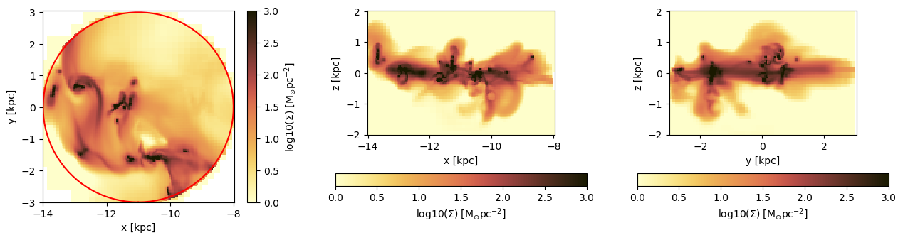
Cylindrical Region: Projections of the sub-region rekated ti a given data center:
proj_z = projection(gas_subregion, :sd, unit=:Msol_pc2, direction=:z, center=[13., 24.,24.], range_unit=:kpc, verbose=false);
proj_y = projection(gas_subregion, :sd, unit=:Msol_pc2, direction=:y, center=[13., 24.,24.], range_unit=:kpc, verbose=false);
proj_x = projection(gas_subregion, :sd, unit=:Msol_pc2, direction=:x, center=[13., 24.,24.], range_unit=:kpc, verbose=false);
The ranges of the plots are now adapted to the given data center:
figure(figsize=(15.5, 3.5))
labeltext=L"\mathrm{log10(\Sigma) \ [M_{\odot} pc^{-2}]}"
theta = LinRange(-pi, pi, 100)

subplot(1,3,1)
im = imshow( log10.(permutedims(proj_z.maps[:sd]) ), cmap=cmap, aspect=proj_z.ratio, origin="lower", extent=proj_z.cextent, vmin=0, vmax=3)
plot( 3. .* sin.(theta), 3 .* cos.(theta), color="red")
xlabel("x [kpc]")
ylabel("y [kpc]")
cb = colorbar(im, label=labeltext)

subplot(1,3,2)
im = imshow( log10.(permutedims(proj_y.maps[:sd]) ), cmap=cmap, origin="lower", extent=proj_y.cextent, vmin=0, vmax=3)

xlabel("x [kpc]")
ylabel("z [kpc]")
ylabel("z [kpc]")
cb = colorbar(im, orientation="horizontal", label=labeltext, pad=0.2);

subplot(1,3,3)
im = imshow( log10.(permutedims(proj_x.maps[:sd]) ), cmap=cmap, origin="lower", extent=proj_x.cextent, vmin=0, vmax=3)

xlabel("y [kpc]")
ylabel("z [kpc]")
ylabel("z [kpc]")
cb = colorbar(im, orientation="horizontal", label=labeltext, pad=0.2);
Cylindrical Region: Get the data outside of the selected region (inverse selection):
gas_subregion = subregion(  gas, :cylinder,
                            radius=3.,
                            height=2.,
                            range_unit=:kpc,
                            center=[13.,:bc,:bc],
                            inverse=true); # direction=:z, by default
[Mera]: 2020-02-18T23:27:29.071
center: [0.2708333, 0.5, 0.5] ==> [13.0 [kpc] :: 24.0 [kpc] :: 24.0 [kpc]]
domain:
xmin::xmax: 0.2083333 :: 0.3333333 ==> 10.0 [kpc] :: 16.0 [kpc]
ymin::ymax: 0.4375 :: 0.5625 ==> 21.0 [kpc] :: 27.0 [kpc]
zmin::zmax: 0.4583333 :: 0.5416667 ==> 22.0 [kpc] :: 26.0 [kpc]
Radius: 3.0 [kpc]
Height: 2.0 [kpc]
Memory used for data table :176.2107973098755 MB
-------------------------------------------------------proj_z = projection(gas_subregion, :sd, :Msol_pc2, center=[:boxcenter], direction=:z, verbose=false);
proj_y = projection(gas_subregion, :sd, :Msol_pc2, center=[:boxcenter], direction=:y, verbose=false);
proj_x = projection(gas_subregion, :sd, :Msol_pc2, center=[:boxcenter], direction=:x, verbose=false);figure(figsize=(15.5, 3.5))
labeltext=L"\mathrm{log10(\Sigma) \ [M_{\odot} pc^{-2}]}"
theta = LinRange(-pi, pi, 100)
subplot(1,3,1)
im = imshow( log10.(permutedims(proj_z.maps[:sd]) ), cmap=cmap, aspect=proj_z.ratio, origin="lower", extent=proj_z.cextent, vmin=0, vmax=3)
plot( 3. .* sin.(theta) .-11, 3 .* cos.(theta), color="red")
xlabel("x [kpc]")
ylabel("y [kpc]")
cb = colorbar(im, label=labeltext)
subplot(1,3,2)
im = imshow( log10.(permutedims(proj_y.maps[:sd]) ), cmap=cmap, aspect=proj_y.ratio, origin="lower", extent=proj_y.cextent, vmin=0, vmax=3)
plot([-3.,3.,3.,-3.,-3.] .-11.,[-2.,-2.,2.,2.,-2.], color="red")
xlabel("x [kpc]")
ylabel("z [kpc]")
cb = colorbar(im, label=labeltext)
subplot(1,3,3)
im = imshow( log10.(permutedims(proj_x.maps[:sd]) ), cmap=cmap, aspect=proj_x.ratio, origin="lower", extent=proj_x.cextent, vmin=0, vmax=3)
plot([-3.,3.,3.,-3.,-3.],[-2.,-2.,2.,2.,-2.], color="red")
xlabel("y [kpc]")
ylabel("z [kpc]")
cb = colorbar(im, label=labeltext);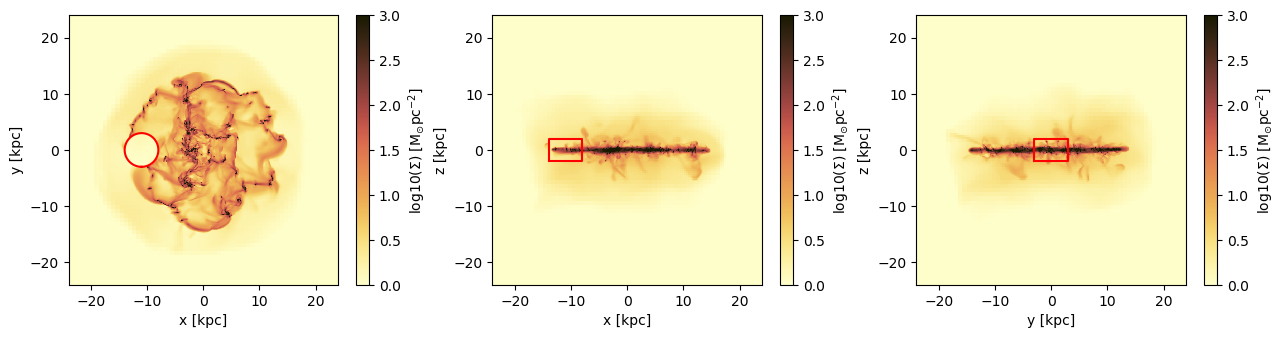
Spherical Region
Create projections of the full box:
proj_z = projection(gas, :sd, unit=:Msol_pc2, center=[:boxcenter], direction=:z, verbose=false);
proj_y = projection(gas, :sd, unit=:Msol_pc2, center=[:boxcenter], direction=:y, verbose=false);
proj_x = projection(gas, :sd, unit=:Msol_pc2, center=[:boxcenter], direction=:x, verbose=false);
100%|███████████████████████████████████████████████████| Time: 0:00:01Spherical Region: The red lines show the region that we want to cutout as a sub-region from the full data:
figure(figsize=(15.5, 3.5))
labeltext=L"\mathrm{log10(\Sigma) \ [M_{\odot} pc^{-2}]}"
theta = LinRange(-pi, pi, 100)

subplot(1,3,1)
im = imshow( log10.(permutedims(proj_z.maps[:sd]) ), cmap=cmap, aspect=proj_z.ratio, origin="lower", extent=proj_z.cextent, vmin=0, vmax=3)
plot( 10. .* sin.(theta) .-11., 10 .* cos.(theta), color="red")
xlabel("x [kpc]")
ylabel("y [kpc]")
cb = colorbar(im, label=labeltext)

subplot(1,3,2)
im = imshow( log10.(permutedims(proj_y.maps[:sd]) ), cmap=cmap, aspect=proj_y.ratio, origin="lower", extent=proj_y.cextent, vmin=0, vmax=3)
plot( 10. .* sin.(theta) .-11., 10 .* cos.(theta), color="red")
xlabel("x [kpc]")
ylabel("z [kpc]")
cb = colorbar(im, label=labeltext)

subplot(1,3,3)
im = imshow( log10.(permutedims(proj_x.maps[:sd]) ), cmap=cmap, aspect=proj_x.ratio, origin="lower", extent=proj_x.cextent, vmin=0, vmax=3)
plot( 10. .* sin.(theta) , 10 .* cos.(theta), color="red")
xlabel("y [kpc]")
ylabel("z [kpc]")
cb = colorbar(im, label=labeltext);
Spherical Region: Cutout the data assigned to the object gas
Select the radius of the sphere in the unit "kpc", relative to the given center [13., 24., 24.]:
gas_subregion = subregion(  gas, :sphere,
                            radius=10.,
                            range_unit=:kpc,
                            center=[13.,:bc,:bc]);
[Mera]: 2020-02-18T23:27:42.261
center: [0.2708333, 0.5, 0.5] ==> [13.0 [kpc] :: 24.0 [kpc] :: 24.0 [kpc]]
domain:
xmin::xmax: 0.0625 :: 0.4791667 ==> 3.0 [kpc] :: 23.0 [kpc]
ymin::ymax: 0.2916667 :: 0.7083333 ==> 14.0 [kpc] :: 34.0 [kpc]
zmin::zmax: 0.2916667 :: 0.7083333 ==> 14.0 [kpc] :: 34.0 [kpc]
Radius: 10.0 [kpc]
Memory used for data table :57.03980731964111 MB
-------------------------------------------------------Spherical Region: Projections of the sub-region.
The coordinates center is the center of the box:
proj_z = projection(gas_subregion, :sd, unit=:Msol_pc2, center=[:boxcenter], direction=:z, verbose=false);
proj_y = projection(gas_subregion, :sd, unit=:Msol_pc2, center=[:boxcenter], direction=:y, verbose=false);
proj_x = projection(gas_subregion, :sd, unit=:Msol_pc2, center=[:boxcenter], direction=:x, verbose=false);
figure(figsize=(15.5, 3.5))
labeltext=L"\mathrm{log10(\Sigma) \ [M_{\odot} pc^{-2}]}"
theta = LinRange(-pi, pi, 100)
subplot(1,3,1)
im = imshow( log10.(permutedims(proj_z.maps[:sd]) ), cmap=cmap, aspect=proj_z.ratio, origin="lower", extent=proj_z.cextent, vmin=0, vmax=3)
plot( 10. .* sin.(theta) .-11., 10 .* cos.(theta), color="red")
xlabel("x [kpc]")
ylabel("y [kpc]")
cb = colorbar(im, label=labeltext)
subplot(1,3,2)
im = imshow( log10.(permutedims(proj_y.maps[:sd]) ), cmap=cmap, aspect=proj_y.ratio, origin="lower", extent=proj_y.cextent, vmin=0, vmax=3)
plot( 10. .* sin.(theta) .-11., 10 .* cos.(theta), color="red")
xlabel("x [kpc]")
ylabel("z [kpc]")
cb = colorbar(im, label=labeltext);
subplot(1,3,3)
im = imshow( log10.(permutedims(proj_x.maps[:sd]) ), cmap=cmap, aspect=proj_x.ratio, origin="lower", extent=proj_x.cextent, vmin=0, vmax=3)
plot( 10. .* sin.(theta) , 10 .* cos.(theta), color="red")
xlabel("y [kpc]")
ylabel("z [kpc]")
cb = colorbar(im, label=labeltext);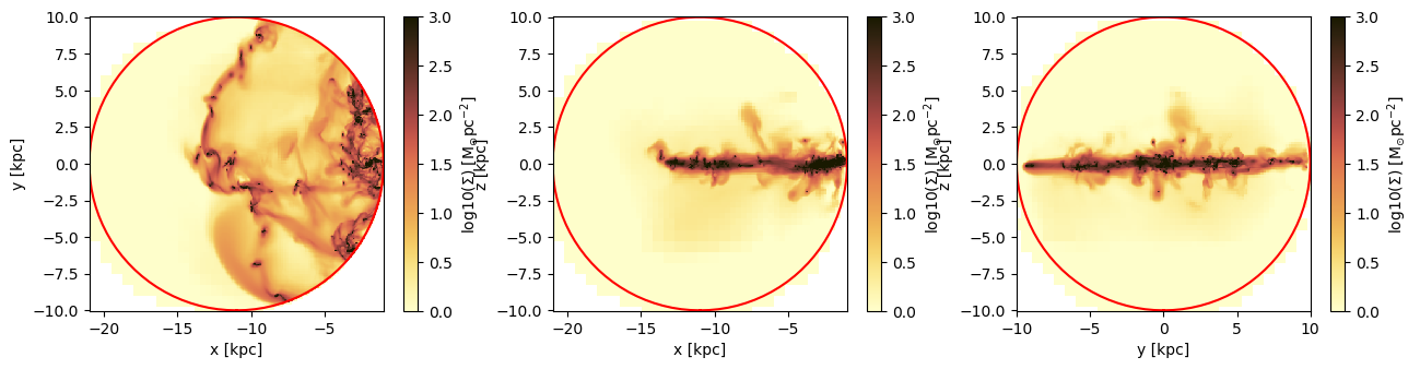
Spherical Region: Get the data outside of the selected region (inverse selection):
gas_subregion = subregion(  gas, :sphere,
                            radius=10.,
                            range_unit=:kpc,
                            center=[13.,:bc,:bc],
                            inverse=true);
[Mera]: 2020-02-18T23:27:46.433
center: [0.2708333, 0.5, 0.5] ==> [13.0 [kpc] :: 24.0 [kpc] :: 24.0 [kpc]]
domain:
xmin::xmax: 0.0625 :: 0.4791667 ==> 3.0 [kpc] :: 23.0 [kpc]
ymin::ymax: 0.2916667 :: 0.7083333 ==> 14.0 [kpc] :: 34.0 [kpc]
zmin::zmax: 0.2916667 :: 0.7083333 ==> 14.0 [kpc] :: 34.0 [kpc]
Radius: 10.0 [kpc]
Memory used for data table :129.1167573928833 MB
-------------------------------------------------------proj_z = projection(gas_subregion, :sd, unit=:Msol_pc2, center=[:boxcenter], direction=:z, verbose=false);
proj_y = projection(gas_subregion, :sd, unit=:Msol_pc2, center=[:boxcenter], direction=:y, verbose=false);
proj_x = projection(gas_subregion, :sd, unit=:Msol_pc2, center=[:boxcenter], direction=:x, verbose=false);figure(figsize=(15.5, 3.5))
labeltext=L"\mathrm{log10(\Sigma) \ [M_{\odot} pc^{-2}]}"
theta = LinRange(-pi, pi, 100)
subplot(1,3,1)
im = imshow( log10.(permutedims(proj_z.maps[:sd]) ), cmap=cmap, aspect=proj_z.ratio, origin="lower", extent=proj_z.cextent, vmin=0, vmax=3)
plot( 10. .* sin.(theta) .-11., 10 .* cos.(theta), color="red")
xlabel("x [kpc]")
ylabel("y [kpc]")
cb = colorbar(im, label=labeltext)
subplot(1,3,2)
im = imshow( log10.(permutedims(proj_y.maps[:sd]) ), cmap=cmap, aspect=proj_y.ratio, origin="lower", extent=proj_y.cextent, vmin=0, vmax=3)
plot( 10. .* sin.(theta) .-11., 10 .* cos.(theta), color="red")
xlabel("x [kpc]")
ylabel("z [kpc]")
cb = colorbar(im, label=labeltext)
subplot(1,3,3)
im = imshow( log10.(permutedims(proj_x.maps[:sd]) ), cmap=cmap, aspect=proj_x.ratio, origin="lower", extent=proj_x.cextent, vmin=0, vmax=3)
plot( 10. .* sin.(theta) , 10 .* cos.(theta), color="red")
xlabel("y [kpc]")
ylabel("z [kpc]")
cb = colorbar(im, label=labeltext);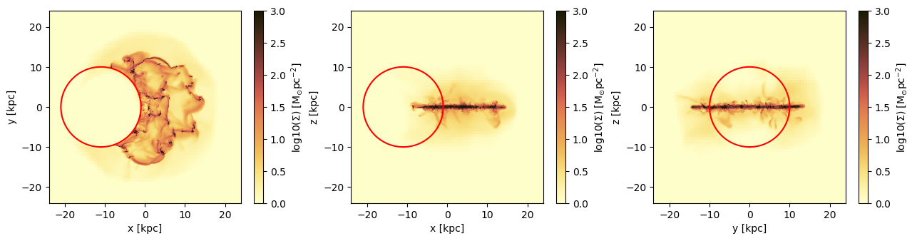
Combined/Nested/Shell Sub-Regions
The sub-region functions can be used in any combination with each other! (Combined with overlapping or nested ranges)
One Example:
comb_region = subregion(gas, :cuboid, xrange=[-8.,8.], yrange=[-8.,8.], zrange=[-2.,2.], center=[:boxcenter], range_unit=:kpc, verbose=false)
comb_region2 = subregion(comb_region, :sphere, radius=12., center=[40.,24.,24.], range_unit=:kpc, inverse=true, verbose=false)
comb_region3 = subregion(comb_region2, :sphere, radius=12., center=[8.,24.,24.], range_unit=:kpc, inverse=true, verbose=false);
comb_region4 = subregion(comb_region3, :sphere, radius=12., center=[24.,5.,24.], range_unit=:kpc, inverse=true, verbose=false);
comb_region5 = subregion(comb_region4, :sphere, radius=12., center=[24.,43.,24.], range_unit=:kpc, inverse=true, verbose=false);proj_z = projection(comb_region5, :sd, unit=:Msol_pc2, center=[:boxcenter], direction=:z, verbose=false);
proj_y = projection(comb_region5, :sd, unit=:Msol_pc2, center=[:boxcenter], direction=:y, verbose=false);
proj_x = projection(comb_region5, :sd, unit=:Msol_pc2, center=[:boxcenter], direction=:x, verbose=false);figure(figsize=(15.5, 3.5))
labeltext=L"\mathrm{log10(\Sigma) \ [M_{\odot} pc^{-2}]}"
theta = LinRange(-pi, pi, 100)
subplot(1,3,1)
im = imshow( log10.(permutedims(proj_z.maps[:sd]) ), cmap=cmap, aspect=proj_z.ratio, origin="lower", extent=proj_z.cextent, vmin=0, vmax=3)
xlabel("x [kpc]")
ylabel("y [kpc]")
cb = colorbar(im, label=labeltext)
subplot(1,3,2)
im = imshow( log10.(permutedims(proj_y.maps[:sd]) ), cmap=cmap, origin="lower", extent=proj_y.cextent, vmin=0, vmax=3)
xlabel("x [kpc]")
ylabel("z [kpc]")
ylabel("z [kpc]")
cb = colorbar(im, orientation="horizontal", label=labeltext, pad=0.2)
subplot(1,3,3)
im = imshow( log10.(permutedims(proj_x.maps[:sd]) ), cmap=cmap, origin="lower", extent=proj_x.cextent, vmin=0, vmax=3)
xlabel("y [kpc]")
ylabel("z [kpc]")
ylabel("z [kpc]")
cb = colorbar(im, orientation="horizontal", label=labeltext, pad=0.2);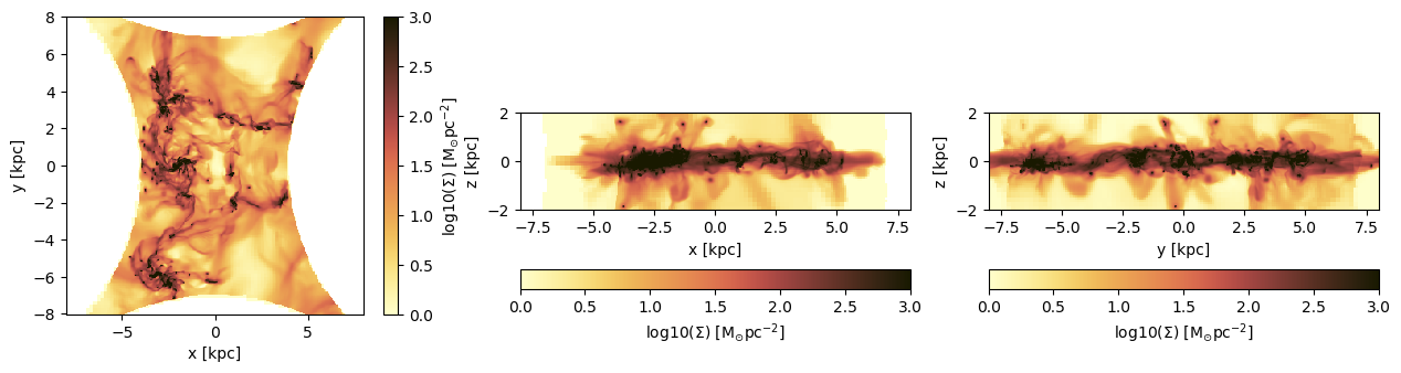
Cylindrical Shell
Create projections of the full box:
proj_z = projection(gas, :sd, unit=:Msol_pc2, center=[:boxcenter], direction=:z, verbose=false);
proj_y = projection(gas, :sd, unit=:Msol_pc2, center=[:boxcenter], direction=:y, verbose=false);
proj_x = projection(gas, :sd, unit=:Msol_pc2, center=[:boxcenter], direction=:x, verbose=false); 100%|███████████████████████████████████████████████████| Time: 0:00:02Cylindrical Shell: The red lines show the shell that we want to cutout as a sub-region from the full data:
figure(figsize=(15.5, 3.5))
labeltext=L"\mathrm{log10(\Sigma) \ [M_{\odot} pc^{-2}]}"
theta = LinRange(-pi, pi, 100)
subplot(1,3,1)
im = imshow( log10.(permutedims(proj_z.maps[:sd]) ), cmap=cmap, aspect=proj_z.ratio, origin="lower", extent=proj_z.cextent, vmin=0, vmax=3)
plot( 10. .* sin.(theta) , 10 .* cos.(theta), color="red")
plot( 5. .* sin.(theta) , 5. .* cos.(theta), color="red", ls="--")
xlabel("x [kpc]")
ylabel("y [kpc]")
cb = colorbar(im, label=labeltext)
subplot(1,3,2)
im = imshow( log10.(permutedims(proj_y.maps[:sd]) ), cmap=cmap, aspect=proj_y.ratio, origin="lower", extent=proj_y.cextent, vmin=0, vmax=3)
plot([-10.,-10.,10.,10.,-10.], [-2.,2.,2.,-2.,-2.], color="red")
plot([-5.,-5,5.,5.,-5.], [-2.,2.,2.,-2.,-2.], color="red", ls="--")
xlabel("x [kpc]")
ylabel("z [kpc]")
cb = colorbar(im, label=labeltext)
subplot(1,3,3)
im = imshow( log10.(permutedims(proj_x.maps[:sd]) ), cmap=cmap, aspect=proj_x.ratio, origin="lower", extent=proj_x.cextent, vmin=0, vmax=3)
plot([-10.,-10.,10.,10.,-10.], [-2.,2.,2.,-2.,-2.], color="red")
plot([-5.,-5,5.,5.,-5.], [-2.,2.,2.,-2.,-2.], color="red", ls="--")
xlabel("y [kpc]")
ylabel("z [kpc]")
cb = colorbar(im, label=labeltext);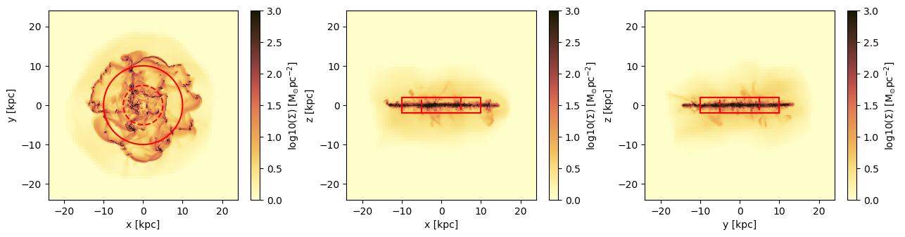
Cylindrical Shell:
Pass the height of the cylinder and the inner/outer radius of the shell in the unit "kpc", relative to the box center [24., 24., 24.]:
gas_subregion = shellregion( gas, :cylinder,
radius=[5., 10.],
height=2.,
range_unit=:kpc,
center=[:boxcenter]); [Mera]: 2020-02-18T23:28:03.834
center: [0.5, 0.5, 0.5] ==> [24.0 [kpc] :: 24.0 [kpc] :: 24.0 [kpc]]
domain:
xmin::xmax: 0.2916667 :: 0.7083333 ==> 14.0 [kpc] :: 34.0 [kpc]
ymin::ymax: 0.2916667 :: 0.7083333 ==> 14.0 [kpc] :: 34.0 [kpc]
zmin::zmax: 0.4583333 :: 0.5416667 ==> 22.0 [kpc] :: 26.0 [kpc]
Inner radius: 5.0 [kpc]
Outer radius: 10.0 [kpc]
Radius diff: 5.0 [kpc]
Height: 2.0 [kpc]
Memory used for data table :53.790066719055176 MB
-------------------------------------------------------proj_z = projection(gas_subregion, :sd, unit=:Msol_pc2, center=[:boxcenter], direction=:z, verbose=false);
proj_y = projection(gas_subregion, :sd, unit=:Msol_pc2, center=[:boxcenter], direction=:y, verbose=false);
proj_x = projection(gas_subregion, :sd, unit=:Msol_pc2, center=[:boxcenter], direction=:x, verbose=false);figure(figsize=(15.5, 3.5))
labeltext=L"\mathrm{log10(\Sigma) \ [M_{\odot} pc^{-2}]}"
theta = LinRange(-pi, pi, 100)
subplot(1,3,1)
im = imshow( log10.(permutedims(proj_z.maps[:sd]) ), cmap=cmap, aspect=proj_z.ratio, origin="lower", extent=proj_z.cextent, vmin=0, vmax=3)
plot( 10. .* sin.(theta) , 10 .* cos.(theta), color="red")
plot( 5. .* sin.(theta) , 5. .* cos.(theta), color="red", ls="--")
xlabel("x [kpc]")
ylabel("y [kpc]")
cb = colorbar(im, label=labeltext)
subplot(1,3,2)
im = imshow( log10.(permutedims(proj_y.maps[:sd]) ), cmap=cmap, origin="lower", extent=proj_y.cextent, vmin=0, vmax=3)
plot([-10.,-10.,10.,10.,-10.], [-2.,2.,2.,-2.,-2.], color="red")
plot([-5.,-5,5.,5.,-5.], [-2.,2.,2.,-2.,-2.], color="red", ls="--")
xlabel("x [kpc]")
ylabel("z [kpc]")
ylabel("z [kpc]")
cb = colorbar(im, orientation="horizontal", label=labeltext, pad=0.2)
subplot(1,3,3)
im = imshow( log10.(permutedims(proj_x.maps[:sd]) ), cmap=cmap, origin="lower", extent=proj_x.cextent, vmin=0, vmax=3)
plot([-10.,-10.,10.,10.,-10.], [-2.,2.,2.,-2.,-2.], color="red")
plot([-5.,-5,5.,5.,-5.], [-2.,2.,2.,-2.,-2.], color="red", ls="--")
xlabel("y [kpc]")
ylabel("z [kpc]")
ylabel("z [kpc]")
cb = colorbar(im, orientation="horizontal", label=labeltext, pad=0.2);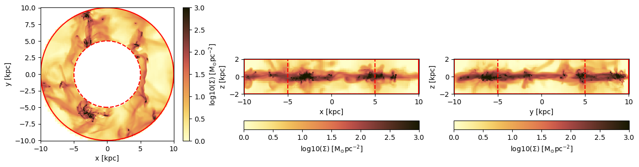
Cylindrical Shell: Get the data outside of the selected shell (inverse selection):
gas_subregion = shellregion(gas, :cylinder,
radius=[5., 10.],
height=2.,
range_unit=:kpc,
center=[:boxcenter],
inverse=true); [Mera]: 2020-02-18T23:28:06.945
center: [0.5, 0.5, 0.5] ==> [24.0 [kpc] :: 24.0 [kpc] :: 24.0 [kpc]]
domain:
xmin::xmax: 0.2916667 :: 0.7083333 ==> 14.0 [kpc] :: 34.0 [kpc]
ymin::ymax: 0.2916667 :: 0.7083333 ==> 14.0 [kpc] :: 34.0 [kpc]
zmin::zmax: 0.4583333 :: 0.5416667 ==> 22.0 [kpc] :: 26.0 [kpc]
Inner radius: 5.0 [kpc]
Outer radius: 10.0 [kpc]
Radius diff: 5.0 [kpc]
Height: 2.0 [kpc]
Memory used for data table :132.36649799346924 MB
-------------------------------------------------------proj_z = projection(gas_subregion, :sd, unit=:Msol_pc2, center=[:boxcenter], direction=:z, verbose=false);
proj_y = projection(gas_subregion, :sd, unit=:Msol_pc2, center=[:boxcenter], direction=:y, verbose=false);
proj_x = projection(gas_subregion, :sd, unit=:Msol_pc2, center=[:boxcenter], direction=:x, verbose=false);figure(figsize=(15.5, 3.5))
labeltext=L"\mathrm{log10(\Sigma) \ [M_{\odot} pc^{-2}]}"
theta = LinRange(-pi, pi, 100)
subplot(1,3,1)
im = imshow( log10.(permutedims(proj_z.maps[:sd]) ), cmap=cmap, aspect=proj_z.ratio, origin="lower", extent=proj_z.cextent, vmin=0, vmax=3)
plot( 10. .* sin.(theta) , 10 .* cos.(theta), color="red")
plot( 5. .* sin.(theta) , 5. .* cos.(theta), color="red", ls="--")
xlabel("x [kpc]")
ylabel("y [kpc]")
cb = colorbar(im, label=labeltext)
subplot(1,3,2)
im = imshow( log10.(permutedims(proj_y.maps[:sd]) ), cmap=cmap, aspect=proj_y.ratio, origin="lower", extent=proj_y.cextent, vmin=0, vmax=3)
plot([-10.,-10.,10.,10.,-10.], [-2.,2.,2.,-2.,-2.], color="red")
plot([-5.,-5,5.,5.,-5.], [-2.,2.,2.,-2.,-2.], color="red", ls="--")
xlabel("x [kpc]")
ylabel("z [kpc]")
cb = colorbar(im, label=labeltext)
subplot(1,3,3)
im = imshow( log10.(permutedims(proj_x.maps[:sd]) ), cmap=cmap, aspect=proj_x.ratio, origin="lower", extent=proj_x.cextent, vmin=0, vmax=3)
plot([-10.,-10.,10.,10.,-10.], [-2.,2.,2.,-2.,-2.], color="red")
plot([-5.,-5,5.,5.,-5.], [-2.,2.,2.,-2.,-2.], color="red", ls="--")
xlabel("y [kpc]")
ylabel("z [kpc]")
cb = colorbar(im, label=labeltext);
Spherical Shell
Create projections of the full box:
proj_z = projection(gas, :sd, unit=:Msol_pc2, center=[:boxcenter], direction=:z, verbose=false);
proj_y = projection(gas, :sd, unit=:Msol_pc2, center=[:boxcenter], direction=:y, verbose=false);
proj_x = projection(gas, :sd, unit=:Msol_pc2, center=[:boxcenter], direction=:x, verbose=false); 100%|███████████████████████████████████████████████████| Time: 0:00:02
100%|███████████████████████████████████████████████████| Time: 0:00:02
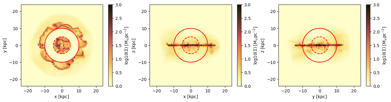
100%|███████████████████████████████████████████████████| Time: 0:00:01Spherical Shell: The red lines show the shell that we want to cutout as a sub-region from the full data:
figure(figsize=(15.5, 3.5))
labeltext=L"\mathrm{log10(\Sigma) \ [M_{\odot} pc^{-2}]}"
theta = LinRange(-pi, pi, 100)
subplot(1,3,1)
im = imshow( log10.(permutedims(proj_z.maps[:sd]) ), cmap=cmap, aspect=proj_z.ratio, origin="lower", extent=proj_z.cextent, vmin=0, vmax=3)
plot( 10. .* sin.(theta) , 10 .* cos.(theta), color="red")
plot( 5. .* sin.(theta) , 5. .* cos.(theta), color="red",ls="--")
xlabel("x [kpc]")
ylabel("y [kpc]")
cb = colorbar(im, label=labeltext)
subplot(1,3,2)
im = imshow( log10.(permutedims(proj_y.maps[:sd]) ), cmap=cmap, aspect=proj_y.ratio, origin="lower", extent=proj_y.cextent, vmin=0, vmax=3)
plot( 10. .* sin.(theta) , 10 .* cos.(theta), color="red")
plot( 5. .* sin.(theta) , 5. .* cos.(theta), color="red", ls="--")
xlabel("x [kpc]")
ylabel("z [kpc]")
cb = colorbar(im, label=labeltext)
subplot(1,3,3)
im = imshow( log10.(permutedims(proj_x.maps[:sd]) ), cmap=cmap, aspect=proj_x.ratio, origin="lower", extent=proj_x.cextent, vmin=0, vmax=3)
plot( 10. .* sin.(theta) , 10 .* cos.(theta), color="red")
plot( 5. .* sin.(theta) , 5. .* cos.(theta), color="red", ls="--")
xlabel("y [kpc]")
ylabel("z [kpc]")
cb = colorbar(im, label=labeltext);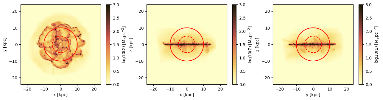
Spherical Shell:
Select the inner and outer radius of the spherical shell in unit "kpc", relative to the box center [24., 24., 24.]:
gas_subregion = shellregion(gas, :sphere,
radius=[5., 10.],
range_unit=:kpc,
center=[24.,24.,24.]); [Mera]: 2020-02-18T23:28:21.357
center: [0.5, 0.5, 0.5] ==> [24.0 [kpc] :: 24.0 [kpc] :: 24.0 [kpc]]
domain:
xmin::xmax: 0.2916667 :: 0.7083333 ==> 14.0 [kpc] :: 34.0 [kpc]
ymin::ymax: 0.2916667 :: 0.7083333 ==> 14.0 [kpc] :: 34.0 [kpc]
zmin::zmax: 0.2916667 :: 0.7083333 ==> 14.0 [kpc] :: 34.0 [kpc]
Inner radius: 5.0 [kpc]
Outer radius: 10.0 [kpc]
Radius diff: 5.0 [kpc]
Memory used for data table :56.55305194854736 MB
-------------------------------------------------------Spherical Shell: Projections of the shell-region.
The coordinates center is the center of the box:
proj_z = projection(gas_subregion, :sd, unit=:Msol_pc2, center=[:boxcenter], direction=:z, verbose=false);
proj_y = projection(gas_subregion, :sd, unit=:Msol_pc2, center=[:boxcenter], direction=:y, verbose=false);
proj_x = projection(gas_subregion, :sd, unit=:Msol_pc2, center=[:boxcenter], direction=:x, verbose=false);
figure(figsize=(15.5, 3.5))
labeltext=L"\mathrm{log10(\Sigma) \ [M_{\odot} pc^{-2}]}"
theta = LinRange(-pi, pi, 100)
subplot(1,3,1)
im = imshow( log10.(permutedims(proj_z.maps[:sd]) ), cmap=cmap, aspect=proj_z.ratio, origin="lower", extent=proj_z.cextent, vmin=0, vmax=3)
plot( 10. .* sin.(theta) , 10 .* cos.(theta), color="red")
plot( 5. .* sin.(theta) , 5. .* cos.(theta), color="red", ls="--")
xlabel("x [kpc]")
ylabel("y [kpc]")
cb = colorbar(im, label=labeltext)
subplot(1,3,2)
im = imshow( log10.(permutedims(proj_y.maps[:sd]) ), cmap=cmap, aspect=proj_y.ratio, origin="lower", extent=proj_y.cextent, vmin=0, vmax=3)
plot( 10. .* sin.(theta) , 10 .* cos.(theta), color="red")
plot( 5. .* sin.(theta) , 5. .* cos.(theta), color="red", ls="--")
xlabel("x [kpc]")
ylabel("z [kpc]")
cb = colorbar(im, label=labeltext)
subplot(1,3,3)
im = imshow( log10.(permutedims(proj_x.maps[:sd]) ), cmap=cmap, aspect=proj_x.ratio, origin="lower", extent=proj_x.cextent, vmin=0, vmax=3)
plot( 10. .* sin.(theta) , 10 .* cos.(theta), color="red")
plot( 5. .* sin.(theta) , 5. .* cos.(theta), color="red", ls="--")
xlabel("y [kpc]")
ylabel("z [kpc]")
cb = colorbar(im, label=labeltext);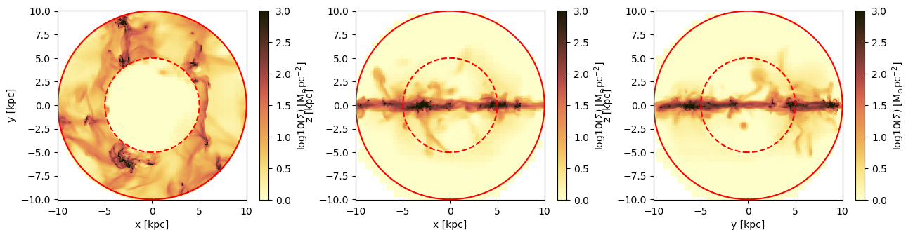
Spherical Shell: Get the data outside of the selected shell-region (inverse selection):
gas_subregion = shellregion(gas, :sphere,
                            radius=[5., 10.],
                            range_unit=:kpc,
                            center=[:boxcenter],
                            inverse=true);
[Mera]: 2020-02-18T23:28:25.267
center: [0.5, 0.5, 0.5] ==> [24.0 [kpc] :: 24.0 [kpc] :: 24.0 [kpc]]
domain:
xmin::xmax: 0.2916667 :: 0.7083333 ==> 14.0 [kpc] :: 34.0 [kpc]
ymin::ymax: 0.2916667 :: 0.7083333 ==> 14.0 [kpc] :: 34.0 [kpc]
zmin::zmax: 0.2916667 :: 0.7083333 ==> 14.0 [kpc] :: 34.0 [kpc]
Inner radius: 5.0 [kpc]
Outer radius: 10.0 [kpc]
Radius diff: 5.0 [kpc]
Memory used for data table :129.60351276397705 MB
-------------------------------------------------------proj_z = projection(gas_subregion, :sd, unit=:Msol_pc2, center=[:boxcenter], direction=:z, verbose=false);
proj_y = projection(gas_subregion, :sd, unit=:Msol_pc2, center=[:boxcenter], direction=:y, verbose=false);
proj_x = projection(gas_subregion, :sd, unit=:Msol_pc2, center=[:boxcenter], direction=:x, verbose=false);figure(figsize=(15.5, 3.5))
labeltext=L"\mathrm{log10(\Sigma) \ [M_{\odot} pc^{-2}]}"
theta = LinRange(-pi, pi, 100)
subplot(1,3,1)
im = imshow( log10.(permutedims(proj_z.maps[:sd]) ), cmap=cmap, aspect=proj_z.ratio, origin="lower", extent=proj_z.cextent, vmin=0, vmax=3)
plot( 10. .* sin.(theta) , 10 .* cos.(theta), color="red")
plot( 5. .* sin.(theta) , 5. .* cos.(theta), color="red", ls="--")
xlabel("x [kpc]")
ylabel("y [kpc]")
cb = colorbar(im, label=labeltext)
subplot(1,3,2)
im = imshow( log10.(permutedims(proj_y.maps[:sd]) ), cmap=cmap, aspect=proj_y.ratio, origin="lower", extent=proj_y.cextent, vmin=0, vmax=3)
plot( 10. .* sin.(theta) , 10 .* cos.(theta), color="red")
plot( 5. .* sin.(theta) , 5. .* cos.(theta), color="red", ls="--")
xlabel("x [kpc]")
ylabel("z [kpc]")
cb = colorbar(im, label=labeltext)
subplot(1,3,3)
im = imshow( log10.(permutedims(proj_x.maps[:sd]) ), cmap=cmap, aspect=proj_x.ratio, origin="lower", extent=proj_x.cextent, vmin=0, vmax=3)
plot( 10. .* sin.(theta) , 10 .* cos.(theta), color="red")
plot( 5. .* sin.(theta) , 5. .* cos.(theta), color="red", ls="--")
xlabel("y [kpc]")
ylabel("z [kpc]")
cb = colorbar(im, label=labeltext);